ISSN: 1992-8645 www.jatit.org E-ISSN: 1817-3195
ANALYSIS OF RADIAL DISTRIBUTION SYSTEM
OPTIMIZATION WITH FACTS DEVICES USING HYBRID
HEURISTIC TECHNIQUE
1
S.VIJAYABASKAR, 2T.MANIGANDAN
1
Associate Professor, Department of Electrical and Electronics Engineering Annapoorana Engineering College, Salem, Tamilnadu, India
2Principal, P.A College of Engineering and Technology, Pollachi, Tamilnadu, India
E-mail:[email protected], [email protected]
ABSTRACT
Distribution networks transport electric energy to the end user from distribution substations. Power utilities are looking for improved power delivery performance. The performance of the delivery system is measured by the power loss of the system. The increase in power loss increases the operating cost of the distribution system. This paper presents an algorithm to minimizing the power loss of the distribution system. Self Adaptive Hybrid Differential Evolution (SaHDE) technique combined with sensitivity factors has been practiced to find the optimal location and the size of FACTS devices to reduce the operating cost of Radial Distribution System (RDS). The locations of the FACTS devices are located by the sensitivity factors. The amount of reactive power component generation/absorption by the FACTS devices at the identified locations has been calculated through SaHDE. The effectiveness of the proposed technique is validated through 10-bus, 34-bus and 85-bus radial distribution systems.
Keywords: Distribution Systems, FACTS, Loss Reduction, Loss Sensitivity Factors, SaHDE.
1
1. INTRODUCTION
For More than five decades, the power loss in distribution system has been reduced through the network reconfiguration and/or by
allocation of capacitor banks. Network
reconfiguration is the process of changing the topology of distribution systems by changing the open/close status of switches. The load at the feeder can be transferred as a result of altering the open/close status of the switches [1 - 3]. However, there are numerous switches in a typical distribution system and the number of possible switching operations is tremendous. Considering this complexity, the capacitor placement has been carried out for loss reduction as an alternative practice. There are various practices have been followed in finding the location of the capacitor banks and the amount of capacitor banks switched on/off to the identified location in the distribution systems. Duran [4] have developed the procedure
for capacitor placement through dynamic
programming and assumed the capacitor sizes as discrete variables. Grainger et al.[5] introduced nonlinear programming for capacitor placement, where variables were treated as continuous. Baran
and Wu [6] proposed a method for capacitor placement using mixed integer programming. The substation level voltage control with dynamic re-sizing of capacitors has been dealt in [7]. Many other optimization methods such as genetic algorithm [8-10], Particle Swarm Optimization [11], Plant Growth Simulation Algorithm [12], tabu search [13], heuristic search techniques [14-16] had been proposed in recent years for capacitor placement problem. Capacitor placement problem has been viewed as multi-constraint problem and the constraints were effectively handled through fuzzy reasoning approach [17]. Farahai et al. [18] has proposed a method combining both capacitor placement and reconfiguration for loss reduction.
ISSN: 1992-8645 www.jatit.org E-ISSN: 1817-3195
In order to overcome the above mentioned short comings, power electronic devices with the improvements in current and voltage handling capabilities (Flexible AC Transmission System-FACTS) have been incorporated. The concept of FACTS devices was originally developed to control reactive power for transmission systems, but it has been introduced recently in distribution systems. Dynamic Voltage Restorer (DVR) is a series connected converter which is used to compensate some of the power quality problems such as voltage sag, voltage unbalance [19-23] which occurs in short duration in millisecond range. In this duration, DVR can inject both active and reactive power to the system for compensation of sensitive loads and active power injection into the system must be provided by energy storage system. Series Static Voltage Restorer (SSVR) was utilized for the improvement of power quality in [24].
In this paper, Static VAR Compensator (SVC), Thyristor-Controlled Series Capacitor (TCSC) and Unified Power Flow Controller (UPFC) are analyzed with distribution system for optimization. The conventional loss sensitivity factors are introduced to identify the optimal location of FACTS devices in the distribution system and the amount of reactive power injection/absorption are fine-tuned with the help of SaHDE in order to accomplish dynamic load variation.
2. PROBLEMFORMULATION
In this paper, the objective of FACTS devices placement in the distribution system is to minimize the total annual cost of the system subject to radial constraint, branch current capacity and bus voltage constraints in which all loads must be energized. The objective function of the problem is mathematically defined in (1),
F = min (AC) (1) Subject to
|Vmin| < |Vi| <|Vmax|
|Imax,j| > |Ij|
where,
AC (Annual Cost)= Ploss,cost+ FACTS cost
Ploss,cost = Energy Loss Cost
FACTScost = FACTS Placement cost
i = 1,2…….nb;
nb = Total number of buses present in RDS
j = 1,2,…….nl;
nl = Total number of lines present in RDS
Vmax= Maximum voltage limit assumed as 1.0 pu
Vmin = Minimum voltage limit assumed as 0.9 pu
2.1 Estimation Power Loss Cost
Figure 1: Single Line Diagram of a Main Feeder
Considering the single line diagram in
figure 1, for calculating the energy loss cost of the distribution system, the following set of load flow equations (2), (3) and (4) are used.
(2) 2 V V Q + P X -Q -Q = Q 2 i 2 i 2 i 2 i 1 + i i, 1 + Li i 1 + i i y − (3) V Q + P ) X + (R + ) Q X + P 2(R -V = V 2 i 2 i 2 i 2 1 + i i, 2 1 + i i, i 1 + i i, i 1 + i i, 2 i 2 1 i+ (4) where,
Pi and Qi are the real and reactive powers that flow
out of bus i;
PLi and QLi are the real and reactive load powers in
bus i
The resistance and reactance of the line section
between buses i and i+1 are denoted by Ri,i+1and
Xi,i+1 respectively.
2 i y
is the total shunt admittance at bus i
The power loss PLoss (i, i+1) of the line
section connecting buses i and i+1 is given in equation (5)
PLoss (i, i+1) = Ri,i+1 2 i 2 i 2 i V Q + P (5)
The power loss PF,Loss of the feeder may be
determined by summing the losses of all line sections of the feeder, given in (6),
PF,Loss = ∑ PLoss (i,i+1) (6)
The total system power loss PT,Loss is the
sum of power losses of all feeders in the system. The total energy loss cost has been calculated as, Ploss_cost=PT,loss * Kp; where Kp is the equivalent
annual cost of power loss in $/(kW-year) assumed as 168 $/(kW-year)
2.2 Estimation of FACTS Devices Cost
The installation cost of FACTS is given by (7). The cost for installation has been taken from [25] and [26].
CSVC = 0.0003S2-0351S+127.38
CTCSC=0.0015S2-7130S+153.75
CUPFC=0.0003S2-2691S+188.22 (7)
where,
2 2
i i
i 1 i Li+1 i,i+1 2 i P +Q P = P - P - R
ISSN: 1992-8645 www.jatit.org E-ISSN: 1817-3195
S - Operating range of the FACTS devices in MVAR
The value of S, calculated using equation (8), S=|Q2|−|Q1| (8)
where,
Q2 - Reactive power flow in the line after
installing FACTS device in MVAR
Q1 - Reactive power flow in the line before
installing FACTS device in MVAR.
The cost is optimized with the following constraint is given in (9) and (10).
-100MVAR ≤ QSVC ≤ 100MVAR (9)
-0.8XL≤ XTCSC ≤ 0.2XL (10)
For UPFC equation (9) and (10) are
considered. Where, XTCSC is the reactance added to
the line by placing TCSC, XL the reactance of the
line where TCSC is located and QSVC is the reactive
power injected at the bus by placing SVC.
3. PROPOSEDALGORITHM
For the FACTS placement, the candidate nodes for placement are determined using the loss sensitivity factors. The amount of reactive power injection through FACTS to the candidate nodes has been determined using the SaHDE algorithm [27].
3.1 Analysis on Finding Optimal Location of FACTS Devices
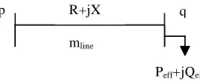
During the early stages, the identification of candidate nodes for FACTS devices placement was carried out through the experience of the engineers and the historical analysis. Then sensitivity analysis has been incorporated in order to reduce the search space and precise solution for indentifying the location. The sensitivity analysis is a conventional procedure to find out the locations with maximum impact on the system real power losses with respect to the node reactive power. The figure 2 illustrates a distribution line with a series impedance of R+jX connected between buses ‘p’ and ‘q’, and an effective load of Peff + jQeff at bus
‘q’. The term ‘eff’ mentioned in the subscript refers the total load connected beyond the referred bus.
Figure 2: Single Line Diagram of a Distribution Line
The active power loss for mth line is given in
equation (11),
2 2
2
( [ ] [ ]) [ ]
P [ ]
( [ ])
eff eff
lineloss
P q Q q R k q
V q
+
= (11)
The loss sensitivity factor can be obtained from equation (12),
2
2 [ ]* [ ]
( [ ]) eff lineloss
eff
Q q R k P
Q V q
∂ =
∂ (12)
With the help of load flow equations, the loss sensitivity factor of all lines are calculated and arranged in descending order of the given system. From this sequence, the end bus of lines which have less than normalized voltage are considered as
weak buses and must need the voltage
improvement at the location.
3.2 SaHDE Algorithm for Identifying FACTS Sizes
The purpose of introduction of SaHDE is to find the optimum amount of reactive power injection through FACTS to be included in the identified optimal location of the distribution system. The pseudocode of the SaHDE algorithm has been given below,
// Pseudocode for SaHDE Let iteration t= 0;
Initialize F_Mean=0.5, F_Variance=0.1, CR_Mean=0.5, CR_Variance=0.1;
Initialize population number (Np) and the maximal iteration
number (Niter),total variable (Nv)
/* Population initialization */ for(pop=1;pop<=Np;pop++)
for( var=1;var<=Nv;var++)
G[pop][var]=getRandom(var_min,var_max,random); do
{
for(pop=1;pop<= Np;pop++)
{
/* Mutation operation*/
j_row=getRandom(1,pop,random); k_row=getRandom (1,pop,random); for( var=1;var<= Nv;var++)
//Calculate F_Gaussian
Gplus[pop][var]=G[pop][var]+F_Gaussian* (G[pop][j_row]-G[pop][k_row]) /* Crossover operation*/
for( var=1;var<= Nv;var++)
{
if(getRandom()>CR_Gaussian) G_plus=G;
}
R+jX
p q
mline
[image:3.612.132.245.632.678.2]ISSN: 1992-8645 www.jatit.org E-ISSN: 1817-3195
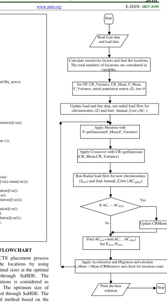
4. COMPUTATIONALFLOWCHART
The optimal FACTS placement process starts with identifying the locations by using sensitivity factors. The optimal sizes at the optimal locations are received through SaHDE. The identified number of locations is considered as variables for the SaHDE. The optimum size of FACTS has been fine tuned through SaHDE. The flowchart for the proposed method based on the
SaHDE algorithm is given in the figure 3.
[image:4.612.199.538.68.681.2]
Figure 3: Flowchart for Reconfiguration through Hybrid SaHDE Algorithm
Update load and line data, run radial load flow for chromosomes (Z) and find Annual_Cost (AC z)
Apply Acceleration and Migration and calculate CR_Mean = Mean (CRMemory) and check for iteration count
Update CRMemory
Stop Start
Read Line data and load data
Calculate sensitivity factors and find the locations. The total numbers of locations are considered as
variables.
Set NP, CR_Variance, CR_Mean, F_Mean, F_Variance, initial population matrix (Z), iter=0
Apply Mutation with F=getGaussian(F_Mean,F_Variance)
Apply Crossover with CR=getGaussian (CR_Mean,CR_Variance)
Run Radial load flow for new chromosomes (Zplus) and find Annual_Cost (ACzplus)
If ACz > ACzplus
Find ACnew=min(ACz , ACzplus)
Set Poloss=Pnloss
Print the best solution
Yes
No /* objective calculation */
if(f(G)>f(Gplus)) {
for( var=1;var<= Nv;var++)
G=Gplus;
CRI_Final[t]=CRI[pop]; }}
Obj_new=min(f(G),f(Gplus)); final_population=pop;
/* Acceleration */ if(Obj_new ==Obj_old) {
for(pop=1;pop<= Np;pop++)
for( var=1;var<= Nv;var++)
G=G-(int) Math.round(α*gradient(Obj_new));
} else
Obj_old=Obj_new; /* Migration */
for( pop=1;pop<=Np;pop++)
{
if(pop!=final_population) for(var=1;var<=Nv;var++)
if(G[pop][var]==G[final_population][var]) ny=ny+0;
else ny=ny+1; }
ro=ny*1.0/(total_loop*(population-1)); ro2=getRandomm();
ro3=getRandomm(); if(ro<0.3)
for( pop=1;pop<=Np;pop++)
if(pop!=final_population) for(var=1;var<=Nv;var++)
{
roo3=((G[final_population][var]- vmin[var])*1.0/(vmax[var]-vmin[var])); if(ro3<roo3)
G[pop][var]=G[final_population][var]+ (ro2*(vmin[var]- G[final_population][var])); else
G[pop][var]=G[final_population][var]+ (ro2*(vmax[var]-
G[final_population][var])); CR_MEAN=Mean (CRI_Final,t);
ISSN: 1992-8645 www.jatit.org E-ISSN: 1817-3195
5. SIMULATIONRESULTS
The proposed algorithm has been
programmed using J2EE servlet programming and run on a P-IV processor with 266 MHz personal computer. The effectiveness of the proposed algorithm has been tested on 10-bus, 34-bus and 85-bus radial distribution systems.
5.1 Test System 1
[image:5.612.114.267.264.309.2]The Test System 1 is a balanced 10-bus radial distribution system [28] shown in figure 4, with the base of 23kV, served from single feeder. The load and line characteristic of the system is shown in table 1.
Figure 4: 10-Bus Radial Distribution System
Table 1: 10-Bus RDS Line and Load Data
Line No.
Start bus
End bus
R (Ω)
X (Ω)
P (kW)
Q (kVAR)
1 1 2 0.1233 0.4127 1840 460
2 2 3 0.0140 0.6057 980 340
3 3 4 0.7463 1.2060 1790 446
4 4 5 0.6984 0.6084 1598 1840
5 5 6 1.9831 1.7276 1610 600
6 6 7 0.9053 0.7886 780 110
7 7 8 2.0552 1.1640 1150 60
8 8 9 4.7953 2.7160 980 130
9 9 10 5.3434 3.0264 1640 200
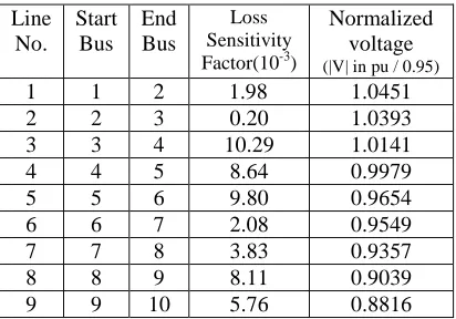
[image:5.612.317.515.297.468.2]With the help of sensitivity analysis the optimal locations were identified. The values of the loss sensitivity factor and normalized voltages are given in table 2.
Table 2: Initial Configuration Sensitivity Factors of 10-Bus RDS
From the table 2, it is clear that the normalized voltages at the buses from 5 to 10 are less than 1.01 pu. These buses are sequenced based on their sensitivity value. The first four buses such as 6, 5, 9 and 10, from the sequence have been considered as sensitive buses and needs voltage control. The FACTS devices are located on those
locations to analyze the performance for
optimization. The impact of the devices with respect to bus voltages and branch currents are shown in the table 3 and table 4 respectively. The tables reveal that the performance of the UPFC is better compared with the other two FACTS devices.
Table 3: Test System 1 Bus Voltages Without and With FACTS Devices
Bus No.
Without FACTS
|Vbus|
(pu)
With SVC |Vbus|
(pu)
With TCSC
|Vbus|
(pu)
With UPFC
|Vbus|
(pu)
1 1.0 1.0 1.0 1.0
2 0.9929 0.9964 0.9961 0.9985
3 0.9873 0.9930 0.9953 0.9973
4 0.9634 0.9844 0.9810 0.9932
5 0.9480 0.9790 0.9810 0.9915
6 0.9171 0.9730 0.9690 0.9895
7 0.9071 0.9715 0.9598 0.9887
8 0.8889 0.9690 0.9429 0.9870
9 0.8586 0.9630 0.9164 0.9857
10 0.8374 0.9555 0.9000 0.9835
Table 4: Test System 1 Branch Currents Without and With FACTS Devices
Line No.
Without FACTS |ILine |
(Amps)
With SVC |ILine |
(Amps)
With TCSC
|ILine |
(Amps)
With UPFC
|ILine |
(Amps)
1 615.25 189.41 568.95 87.60
2 532.93 145.25 487.55 75.71
3 487.30 139.31 444.46 73.08
4 404.72 137.70 366.16 71.43
5 309.71 58.81 290.75 56.13
6 229.72 34.16 215.34 17.53
7 191.97 33.88 179.69 17.34
8 135.82 33.63 126.67 17.12
9 85.77 36.52 79.79 18.55
The power loss and annual operating cost of the distribution system with influence of capacitors and FACTS devices are compared in the table 5.
Line No.
Start Bus
End Bus
Loss Sensitivity Factor(10-3)
Normalized voltage
(|V| in pu / 0.95)
1 1 2 1.98 1.0451
2 2 3 0.20 1.0393
3 3 4 10.29 1.0141
4 4 5 8.64 0.9979
5 5 6 9.80 0.9654
6 6 7 2.08 0.9549
7 7 8 3.83 0.9357
8 8 9 8.11 0.9039
[image:5.612.85.291.573.717.2]ISSN: 1992-8645 www.jatit.org E-ISSN: 1817-3195
Table 5: Comparison of Results with Capacitor Placement and FACTS Devices
Para meters
With out Comp
ensat ors
With Capac itor Place ment [16]
With SVC
With TCSC
With UPFC
Power loss (kW)
783.77 704.883 55.28 671.27 18.96
Annual operating
cost $/year
131,674 119,420 121,547 228,354 121,547
Min. Voltage
in pu.
0.8374 0.9010 0.9555 0.9000 0.9835
From the table 5, the following
observations were found,
i. Compared with static shunt capacitors, the
loss reduction through the FACTS devices is better.
ii. Compared with static shunt capacitors, the
minimum bus voltage is improved with SVC and UPFC.
iii. Compared with FACTS devices, the
annual operating cost through the static shunt capacitors is reduced with small margin (it is obvious that the operating cost of the FACTS devices are more compared with static devices)
iv. Compared with SVC and TCSC, the
performance of the UPFC is good.
5.2 Test System 2
[image:6.612.87.297.130.340.2]The proposed method has been tested with 34-bus balanced radial distribution system [29], shown in figure 5.
Figure 5: 34-Bus Radial Distribution System
As per the sensitivity analysis, the
sensitive buses are identified. The constant Kp is
assumed as the same value as followed for test system 1. For this test system, the lines 17, 20 and 18 are selected as optimal locations for the series voltage regulation and the buses 19, 22 and 20 are selected for reactive power injection/absorption. The proposed method reduces the power loss from 221.67kW to 81.32kW, and maintains the bus voltages well above minimum value. The optimal amount of reactance at the locations 17, 20 and 18,
are -0.33 Ω, 0.06 Ω and -0.27 Ω respectively. The
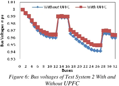
[image:6.612.315.513.304.447.2]optimal amount of reactor at the buses is 1396kVAR, 728kVAR and 26kVAR respectively. The bus voltages with and without UPFC has been shown in the figure 6. It shows that bus voltages of the weaker buses 8, 9 and 10 are improved. The total operating cost of the distribution system is 56233.19$/year.
Figure 6: Bus voltages of Test System 2 With and
Without UPFC
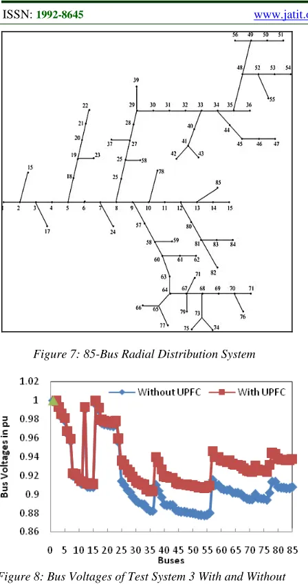
5.3 Test System 3
The proposed method has been validated further by implementing to 85-bus balanced radial distribution system [30], shown in figure. 7. The sensitive buses 8, 58 and 7 were identified through
sensitivity analysis for reactive power
injection/absorption. The associated lines for the series reactance locations are 16, 64 and 14. The
constant Kp is assumed as the same value as
[image:6.612.92.301.546.669.2]ISSN: 1992-8645 www.jatit.org E-ISSN: 1817-3195
[image:7.612.89.313.71.495.2]Figure 7: 85-Bus Radial Distribution System
Figure 8: Bus Voltages of Test System 3 With and Without UPFC
6. CONCLUSION
In this paper, SaHDE algorithm along with sensitivity factors has been proposed to solve the reactive power control through FACTS devices. The purpose of the loss sensitivity factors is to identify the sensitive buses of the distribution system. With the integration of SaHDE, the optimal
values of reactive power component
generation/absorption by the FACTS devices at the identified locations were calculated. Furthermore, the suitability of the FACTS devices such as SVC, TCSC and UPFC were analyzed for distribution system optimization. From the results, it is absorbed that UPFC performs better in maintaining bus voltages above the minimum limit and the significant reduction of annual operating cost, compared with other FACTS devices. With the above observations, it is very well understood that
the presence of UPFC in the distribution system greatly improves the efficiency. Besides, the improvements in the voltages at the buses provide opportunity for expansion planning and protection during faulted conditions. The main advantages of the proposed algorithm with the previous works addressed are that, evade of heavy numerical computing, promising the global optimum, solution for the control parameters, quick searching for optimal solution and suitable for dynamic load patterns.
REFERENCES
[1] Sathiskumar. M, Nirmalkumar. A,
Thiruvenkadam. S, and Lakshminarasimman. L, “Feeder Reconfiguration and Service Restoration in Distribution Networks Through Fusion Technology: Part 2”, Australian
Journal of Electrical and Electronics
Engineering, vol.8, no. 3, 2011, pp. 219-230. [2] C. Wang and H.Z. Cheng, “Optimization of
Network configuration in Large distribution
systems using plant growth simulation
algorithm”, IEEE Trans. Power Syst., vol.23, no. 1, 2008, pp. 119-126.
[3] A. C. B. Delbem, A. C. P. L. F. Carvalho, and N. G. Bretas, “Main chain representation for evolutionary algorithms applied to distribution system reconfiguration”, IEEE Trans. Power Syst., vol. 20, no. 1, 2005, pp. 425–436. [4] Duran H. “Optimum number, Location and
size of shunt capacitors in radial distribution feeders: a dynamic programming approach”, IEEE Trans. Power Apparat. Syst., vol.87, no.9, 1983, pp.1769–1774.
[5] Grainger JJ, and Lee SH, “Optimum size and location of shunt capacitors for reduction of losses on distribution feeders”, IEEE Trans Power Apparat. Syst., vol.100, no.3, 1981, pp.1105–1118.
[6] Baran ME and Wu FF, “Optimal capacitor placement on radial distribution system”, IEEE Trans Power Deliv., vol.4, no.1, 1989, pp.725– 734.
[7] Baghzouz Y, and Ertem S, “Shunt capacitor sizing for radial distribution feeders with distorted substation voltages”, IEEE Trans. Power Deliv., vol.5, 1990, pp.650–657. [8] Sundhararajan S, Pahwa A, “Optimal selection
of capacitors for radial distribution systems using genetic algorithm”, IEEE Trans. Power Syst., vol.9, no.3, 1994, pp.1499–507.
ISSN: 1992-8645 www.jatit.org E-ISSN: 1817-3195
distribution systems using a genetic
algorithm”, in Proc. IEEE Power Eng. Soc. T&D Latin Amer. Conf., 2002.
[10] Das D., “Reactive power compensation for radial distribution networks using genetic algorithms,” Electrical Power Energy Syst., vol. 24, 2002, pp.573–581.
[11] Prakash K, and Sydulu M., “Particle swarm optimization based capacitor placement on radial distribution systems”, IEEE power engineering society general meeting; 2007, pp. 1–5.
[12] Srinivasas Rao R, Narasimham S.V.L, and
Ramalingaraju M, “Optimal capacitor
placement in a radial distribution system using
Plant Growth Simulation Algorithm”,
Electrical Power Energy Syst., vol.33, 2011, pp.1133-1139.
[13] Yann-Chang Huang et al., “Solving the Capacitor Placement Problem in a Radial Distribution System Using Tabu Search Approach”, IEEE Transactions on Power Systems, Vol. 11, No. 4, 1996, pp.1868-1873. [14] Mekhamer SF et al., “New heuristic strategies
for reactive power compensation of radial distribution feeders”, IEEE Trans. Power Deliv., vol.17, no.4, 2002, pp.1128–1135. [15] Chis M, Salama MMA, and Jayaram S.,
“Capacitor placement in distribution system using heuristic search strategies”, IEE Proc-Gener. Transm. Distrib., vol. 44, no.3, 1997, pp.225–230.
[16] S. Vijayabaskar, and T. Manigandan,
“Capacitor Placement in Radial Distribution System Loss Reduction using Self Adaptive Hybrid Differential Evolution and Loss Sensitivity Factors”, European Journal of Scientific Research, Vol. 87, No. 2, 2012, pp.201-211.
[17] Su CT, and Tsai CC., “A new fuzzy reasoning approach to optimum capacitor allocation for primary distribution systems”, In Proceeding of the IEEE on industrial technology conference; 1996, pp. 237–41.
[18] Farahai, Behrooz, and Hossein,
“Reconfiguration and capacitor placement simultaneously for energy loss reduction based on an improved reconfiguration method”, IEEE Trans. Power Syst., vol. 27, no. 2, 2012, pp. 587-595.
[19] M.H. Haque, “Compensation of distribution system voltage sag by DVR and D-STATCOM”, 2001, IEEE Porto Power Tech Conference, Vol. 1, 2001, pp. 223-228.
[20] A. Ghosh, and G. Ledwich, “Compensation of distribution system voltage using DVR”, IEEE Transactions on Power Delivery, Vol.17, 2002, pp.1030 – 1036.
[21] H. Ding, S. Shuangyan, D. Xianzhong and G. jun, “A Novel Dynamic Voltage Restore and Its Unbalance Control Strategy Based on Spaced Vector PWM”, ELSEVIER, Electric Power Systems Research, vol. 24, 2001, pp.693–699.
[22] M. Chawla, A. Rajvanshy, A. Ghosh, and A. Joshi, “Distribution bus voltage control using DVR under the supply frequency variations”, IEEE Power India Conference, 2006, pp. 272-277.
[23] P.T. Nguyen and T.K Saha, “Dynamic voltage restorer against balanced and unbalanced voltage sags: modelling and simulation”, IEEE Power Engineering Society General Meeting, Vol.1, 2004, pp.639- 644.
[24] M. Fotuhi-Firuzabad, H. A. Shayanfar, M. Hosseini, “Modeling of Series Static Voltage Restorer (SSVR) in Distribution Systems Load Flow”, IEEE Conference (978-1-4244-1583-0/07), 2007.
[25] L.J. Cai, I. Erlich, “Optimal choice and allocation of FACTS devices using genetic
algorithms”, Proceedings on Twelfth
Intelligent Systems Application to Power Systems Conference,2003, pp. 1–6.
[26] L.J. Cai, I. Erlich, “Optimal choice and allocation of FACTS devices in deregulated electricity market using genetic algorithms”, IEEE Conference (0-7803-8718-X/04), 2004.
[27] M. Sathiskumar, A. Nirmalkumar, S.
Thiruvenkadam & L. Lakshminarasimman, “A self adaptive hybrid differential evolution algorithm for phase balancing of unbalanced distribution system”, International Journal of Electrical Power and Energy Systems, vol. 42, 2012, pp. 91-97.
[28] Baghzouz Y, Ertem S., “Shunt capacitor sizing for radial distribution feeders with distorted substation voltages”, IEEE Trans. Power Deliv., vol.5,1990, pp.650–657.
[29] Chis M, Salama MMA, and Jayaram S., “Capacitor placement in distribution system using heuristic search strategies”, IEE Proc-Gener. Transm. Distrib., vol.144, no.3, 1997, pp.225–30.