ADAPTATION OF THE HARMONY SEARCH ALGORITHM
TO SOLVE THE TRAVELLING SALESMAN PROBLEM
1
MORAD BOUZIDI, 2MOHAMMED ESSAID RIFFI
Laboratory Of Matic, Mathematics & Computer Science Dept.
Faculty Of Sciences, Chouaïb Doukkali University El Jadida, Morocco
E-mail : 1[email protected], 2[email protected]
ABSTRACT
The travelling salesman problem (TSP) is a discrete combinatorial optimization problem; it allows us to solve a set of problems in the real world in various fields. This article presents a new meta-heuristic adaptation to solving this problem. The numerical results are applied to a set of instances of TSPLIB we showing us the effectiveness of the adaptation of the harmony search algorithm band compared to other approaches in terms of quality of the solution, the search time, and the improvement of the results in terms of the reduction in the percentage of errors.
Keywords: Combinatorial Optimization, Meta-Heuristic, Travelling Salesman Problem, Harmony
Search Algorithm, Local Search.
1. INTRODUCTION
The travelling salesman problem is a famous problem of operational research. Indeed, this problem consist of finding the shortest path to travel from one seller, which begins by a departure city, passing only once through each city and coming back, to the city of departure. The objective is to find the Hamiltonian cycle in both minimal time and cost.
There are several application fields, such as logistics [1], scheduling [2], transportation [3]. For example; finding the shortest path for school buses, factories personal transportation, or for trucks used to transport goods. The travelling salesman problem (TSP) belongs to the class of NP-complete problems [4], non-polynomial complexity.
Many methods have been developed to solve the TSP problem as the descent [5], simulated annealing [6], tabu [7], and meta-heuristics methods that are generally high levelled strategies that are based on probabilistic decisions made during the research, such genetic algorithm [8] and ant algorithm [9].
This paper presents an adaptation of the harmony search algorithm to solve this problem. This article is organized as follows. In section 2, a formulation of the travelling salesman problem, in Section 3 a definition of the harmony search algorithm, in Section 4 the strategy of adapting the algorithm for
TSP problem, Section 5 presents the results and debate about the algorithm, and finally, conclusions.
2. TRAVELLING SALESMAN PROBLEM
The travelling salesman problem was mentioned for the first time in 1930 by the mathematician Karl Menger [10]. Solving this problem consists of establishing the minimal length of the Hamiltonian cycle in a complete and undirected graph in which each vertex represents a city and each edge represents a path. Each path has a cost that represents the distance to get from one vertex to another.
The travelling salesman problem is composed of a set of variables:
|| , ଵஸஸ
ଵஸஸ
, the matrix to trace the path as:
1, 0,
The problem consists of minimizing the length of Hamiltonian cycle:
ୀଵ
1
ୀଵ
ୀଵ
1 , !! є "1, … , $ 2
ୀଵ
1 , !! є "1, … , $ 3
And
єௌ єௌ
є ', !! ' є ( 4
Search the constraint equation 2 (or 3) has been proposed to ensure that every city has a single successor (pre-successor), the constraint equation 4 in order to prohibit the solutions that are sub-cycle (which passes only a subset of n city).
3. HARMONY SEARCH ALGORITHM
The harmony search algorithm (HS) is a meta-heuristic approach inspired by natural processes of musical performances. It was developed by Geem and al. [11] in 2001, and has been studied by many researchers as Lee and al. [12] Geem. [13] Saka [14, 15], and Erdal Saka [16] and Degertekin [17, 18]. The algorithm consists of finding a perfect state of harmony in a musical orchestra in which each musician plays a note, to find a better harmony. In a similar manner, each musician plays a note in the broadest possible to form a band with other musicians. If all the notes played by all the musicians are seen as harmonious, then it is stored in the memory of each of the musicians in order to get the same optimal result for the next time.
The HS algorithm consists of five main steps. The following algorithm (Algorithm.1) represents the optimization of the search algorithm band procedure.
Step 1.Initialize the algorithm parameters. Step 2.Initialize the harmony memory. Step 3.Improvise a new harmony. Step 4.Update the Harmony Memory. Step 5.Check the stopping criterion.
These steps are described in the next five subsections.
3.1 Initialization of the Parameters:
In this step, we initialize the algorithm parameters: the number of solutions generated (HMS), the rate of memory considered (HMCR), the adjustment rate (PAR) and the other stopping criteria like the maximal number of iterations.
3.2 Initialization of the Harmony Memory:
The initiation of the band memory HM is to generate the HMS solutions in a random way; each
x solution is consisting of N elements. For each solution the objective function f is calculated, the equation (5) presents the general structure of the HM. ଵ ଵ ଵ ଶ ⋮ ⋮ ଵ ுெௌିଵ ଵ ுெௌ ଶ ଵ ଶ ଶ ⋮ ⋮ ଶ ுெௌିଵ ଶ ுெௌ … … … … … … ିଵ ଵ ିଵ ଶ ⋮ ⋮ ିଵ ுெௌିଵ ିଵ ுெௌ ଵ ଶ ⋮ ⋮ ுெௌିଵ ுெௌ → → → → → → ଵ ଶ ⋮ ⋮ ுெௌିଵ ுெௌ (5)
3.3 Improvising a New Harmony:
A new solution x = (xଵ, xଶ, … , x୬) using two parameters: (i) rate regardless of the harmony memory HMCR, (ii) rate setting step PAR. These parameters help the algorithm obtain solutions locally or globally improved. The solution is built for each element of the new solution as follows:
x୧ ∈ ,-x୧ ଵ, x
୧ ଶ, … , x
୧
ୌୗ. with probability HMCR
Xୱ with probability 1 ? HMCR Where Xs is the set of all possible elements for each variable.
Each variable obtained by the consideration of the memory is examined to determine if it should be adjusted or not. Using the second parameter the pitch adjustment rate (PAR) which controls the search for better solutions. PAR is used as follows:
x୧ x୧ bw ∗ u1,1 with probability PAR x୧ with probability 1 PAR Where bw is a bandwidth of distance and u (-1.1) is distributed uniformly between -1 and 1.
3.4 Update the Harmony Memory:
The new generated harmony replaces the worst one stored in the memory band (HM), only if its physical condition (measured in terms of the objective function) is better than the worst harmony.
3.5 Checking the Stopping Criterion:
The execution of the algorithm terminates when the maximum number of repetitions is reached or when the algorithm finds the right harmony.
4. ADAPTATION OF THE HARMONY SEARCH ALGORITHM TO THE TRAVELLING SALESMAN PROBLEM
The search algorithm is based on the following parameters:
HMS : The size of the solutions memory (HM).
Algorithm.1 : Search Harmony Algorithm.
HMCR : Probability to choose a city in the
memory.
PAR : Probability of adjustment to choose a neighbours city.
The first phase of adaptation shown in Algorithm.2 is to initialize the HMCR, PAR, and HMS settings. The second phase consists of initializing the HM harmony memory of
the HM solutions in a random way so that each solution represents an Hamiltonian cycle of cities. The third phase consists of starting to look for a solution that depends on values of parameters until the stop condition is satisfied.
In this adaptation, the algorithm stops looking for new solutions when the number of iterations of searches exceeds the maximal number, or when the algorithm manages to find the optimum of the problem’s instance.
The next step is to generate a new cycle. For each index from 1 to n (number of cities) of the new solution randomly selects a number between 0 and 1 (PHMCR). If the number is strictly less than HMCR, then memory is considered, otherwise the algorithm choses a city in a random way. If the memory is considered then the algorithm selects a city from the memory. Once the city is obtained, we generate another random number between 0 and 1 (PPAR), if the latter is less than the value of the adjustment’s parameter PAR, then the algorithm replaces the city obtained by one of his neighbours. Once the city is recovered, the algorithm inserts it into the current index of the new solution. Before each insertion into the new solution, the algorithm
checks for the selected city, to avoid closing the cycle.
Algorithm.2 : Adaptation of the Algorithm Begin
Initialization of the parameters: HMS, HMCR and PAR. Initialization of the HM memory by HMS solutions.
While ((iteration <maximum number of iterations) and
(the algorithm has not reached the best problem)) do For each i ∈∈∈∈ cities do
If (PHMCR <HMCR) then
Choose a city from the HM column i. If (PPAR<PAR) then
Replace the selected city with one of its neighbours.
end If else
Select a city randomly. end If
Place the chosen city in the current location of the new cycle.
end for
Improve the new solution by the local search method.
Update HM memory.
end while
Return the best solution of the HM. End.
determines the position of the poor solution of the memory, increases the number of iterations, then restarts the process.
The approach of this article is applied to solve the TSP problem using the local search method as the descent method.
5. RESULTS AND DEBATE
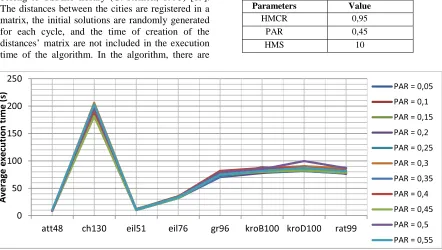
The adaptation of the proposed algorithm is coded into a program language C+ + on visual studio 2010, the results are executed on a computer Intel (R) Core (TM) 2 Duo CPU [email protected] 2.10GHz and 2.00 GB of RAM. Instances used belong to TSPLib library (G. Reinelt, 1995) [19]. The distances between the cities are registered in a matrix, the initial solutions are randomly generated for each cycle, and the time of creation of the distances’ matrix are not included in the execution time of the algorithm. In the algorithm, there are
three key parameters that influence the performance results: the size of the memory band (HMS), the rate of the memory consideration (HMCR) and the rate of the pitch adjustment (PAR). The values of the HMS and HMCR parameters used are 0.95 and 10 [20]. for the value of the rate adjustment we applied a combination of values in the interval ]0,6[ with steps of 0.05 , which is shown on the figure 1 (Figure 1). it shows the variation of the average execution time of each PAR value for 8 TSPLib bodies , and from the results (Figure 2) we find that the 0.45 value minimizes the execution time. So the values of the chosen used parameters are:
Table 1: Values of the Adaptation Parameters
Parameters Value
HMCR 0,95
PAR 0,45
[image:4.612.90.532.270.520.2]HMS 10
Figure 1: The Variation Of The Average Execution Time Of Each PAR Value.
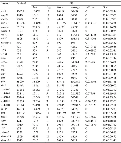
Table 2 shows the effect of adaptation and the local search. Before showing the results, we will compare the best solutions obtained by the different methods used in the adaptation for 10 iterations on instances of the represented problem, which shows the obtained result by the local search method and the adaptation of the algorithm. The results of the adaptation are presented in table 3. The first column represents the best length obtained, the second indicates the number of times the algorithm reaches the optimum problem, the third shows the worst length obtained, while the fourth represents the average length of the iterations, the fifth is about the relative error, and the last column is the average
execution time. The relative error is calculated as follows:
[image:4.612.313.522.646.727.2]– ′! " # ′! " # $ %&& %
Table 2: Results of the Descent Method and the Adaptation of the Harmony Search Algorithm
Instance Optimal Local search
Harmony search
att48 10628 10824 10628
ch150 6528 6969 6549
gr96 55209 56558 55209
hk48 11461 11470 11461
kroA100 21282 21827 21282
0 50 100 150 200 250
att48 ch130 eil51 eil76 gr96 kroB100 kroD100 rat99
A
v
e
ra
g
e
e
x
e
cu
ti
o
n
t
im
e
(
s)
PAR = 0,05
PAR = 0,1
PAR = 0,15
PAR = 0,2
PAR = 0,25
PAR = 0,3
PAR = 0,35
PAR = 0,4
PAR = 0,45
PAR = 0,5
kroB100 22141 22979 22141
kroD100 21294 21488 21294
kroE100 22068 22437 22073
[image:5.612.97.516.174.670.2]st70 675 691 675
Table 3. The Results of the Harmony Adaptation Proposed for TSP
Instance Optimal HS
Best Nbest Worst Average % Error Time
att48 10628 10628 10 10628 10628 0 00:00:08:54
bayg29 1610 1610 10 1610 1610 0 00:00:02:07
bays29 2020 2020 10 2020 2020 0 00:00:02:03
bier127 118282 118498 1 119165 11843.5 0.474713 00:02:54:78
brazil58 25395 25395 10 25395 25395 0 00:00:16:28
burma14 3323 3323 10 3323 3323 0 00:00:00:29
ch130 6110 6110 1 6171 6143.1 0.541735 00:03:01:54
ch150 6528 6553 1 6609 6583.1 0.844056 00:06:30:38
dantzig42 699 699 10 699 699 0 00:00:05:82
eil51 426 426 7 427 426.3 0.070423 00:00:10:46
eil76 538 538 3 543 540.2 0.408922 00:00:32:41
eil101 629 630 1 642 636.9 1.25596 00:01:15:10
fri26 937 937 10 937 937 0 00:00:01:36
gil262 2378 2435 1 2446 2438.4 2.53995 00:26:56:00
gr17 2085 2085 10 2085 2085 0 00:00:00:55
gr21 2707 2707 10 2707 2707 0 00:00:00:88
gr24 1272 1272 10 1272 1272 0 00:00:01:45
gr48 5046 5046 10 5046 5046 0 00:00:09:18
gr96 55209 55209 1 55436 55334.3 0.226956 00:01:11:85
hk48 11461 11461 10 11461 11461 0 00:00:09:02
kroA100 21282 21282 10 21282 21282 0 00:01:22:15
kroB100 22141 22141 5 22211 22158.2 0.077684 00:01:19:68
kroC100 20749 20749 10 20749 20749 0 00:01:23:26
kroD100 21294 21294 3 21389 21338.4 0.208509 00:01:22:65
kroE100 22068 22068 3 22106 22084.6 0.075222 00:01:22:18
lin105 14379 14379 10 14379 14379 0 00:01:35:71
pr76 108159 108159 10 108159 108159 0 00:00:35:58
pr107 44303 44303 5 44347 44317.9 0.033632 00:01:35:66
rat99 1211 1215 1 1220 1217.8 0.561519 00:01:18:20
rd100 7910 7910 4 7914 7911.4 0.017699 00:01:21:62
st70 675 675 10 675 675 0 00:00:28:18
swiss42 1273 1273 10 1273 1273 0 00:00:06:93
ulysses16 6859 6859 10 6859 6859 0 00:00:00:73
ulysses22 7013 7013 10 7013 7013 0 00:00:01:45
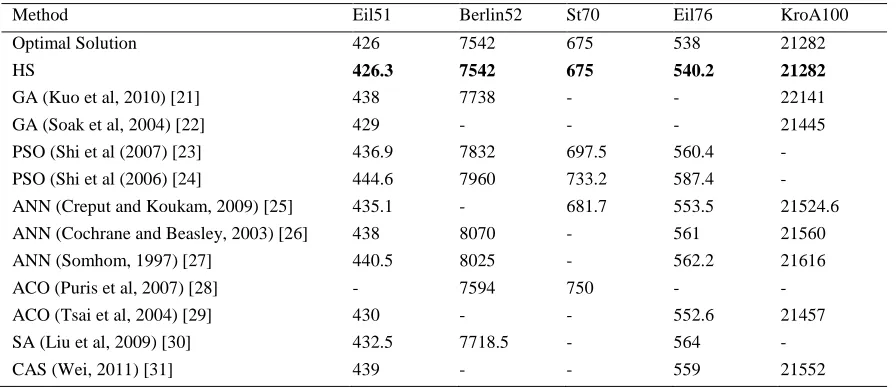
After the evaluation of the adaptation on a set of instances of the problem, Table 4 compares its performance versus other existing algorithms such as Genetic Algorithm (GA), particle swarm
Table 4. Calculation of the Average Results of Many Meta-Heuristiques Approches
Method Eil51 Berlin52 St70 Eil76 KroA100
Optimal Solution 426 7542 675 538 21282
HS 426.3 7542 675 540.2 21282
GA (Kuo et al, 2010) [21] 438 7738 - - 22141
GA (Soak et al, 2004) [22] 429 - - - 21445
PSO (Shi et al (2007) [23] 436.9 7832 697.5 560.4 -
PSO (Shi et al (2006) [24] 444.6 7960 733.2 587.4 -
ANN (Creput and Koukam, 2009) [25] 435.1 - 681.7 553.5 21524.6
ANN (Cochrane and Beasley, 2003) [26] 438 8070 - 561 21560
ANN (Somhom, 1997) [27] 440.5 8025 - 562.2 21616
ACO (Puris et al, 2007) [28] - 7594 750 - -
ACO (Tsai et al, 2004) [29] 430 - - 552.6 21457
SA (Liu et al, 2009) [30] 432.5 7718.5 - 564 -
CAS (Wei, 2011) [31] 439 - - 559 21552
6. CONCLUSION
We have implemented a matching harmony search algorithm to solve the problem of salesmen in order to find the best optimized path way. An empirical study has been done in order to determine the impact of the parameters of harmony search algorithm upon solutions’ quality. The ability of the algorithm was demonstrated using multiple instances of the TSP problem, and it was concluded that the proposed adaptive algorithm is more effective in finding the best solutions, and also its performance compared to other optimization methods such as genetic algorithm and simulated annealing and ant. Thus, we believe that our adaptation will be adapted to solve other optimization because of its fast and reliable convergence.
7. REFERENCES
[1] FILIP, E., M. OTAKAR, The Travelling Salesman Problem and its Application in Logistic Practice, WSEAS Transactions on Business and Economics, Vol. 8, no. 4, 2011, pp. 163-173
[2] Gavish, B. and Graves S. C. The Travelling Salesman Problem and Related Problems. Working Paper OR-078-78, Operations Research Center, MIT, Cambridge, MA, 1978.
[3] Ungureanu, Valeriu, Travelling Salesman Problem with Transportation. Computer Science Journal of Moldova, Vol. 14, no. 2, 2006.
[4] G.Gutiand A.Punnen, editors, The Traveling Salesman Problem and its Variations, Kluwer Academic Publishers, 2002, pp. 369–443.
[5] Christos Voudouris, Edward Tsang , Guided local search and its application to the traveling salesman problem, European Journal of Operational Research, Vol.113, no. 2, 1999, pp. 469-499.
[6] C.S. Jeong, M.H. Kim, Fast parallel simulated annealing for traveling salesman problem on SIMD machines with linear interconnections, Parallel Comput., Vol. 17, 1991, pp. 221–228
[7] C.-N.Fiechter, A parallel Tabu search algorithm for large traveling salesman problems, Discrete Appl. Math., Vol. 51, 1994, pp. 243– 267.
[8] M. Albayrak, N. Allahverdi, Development a new mutation operator to solve the traveling salesman problem by aid of genetic algorithms, Expert Syst. Appl., Vol. 38, 2011, pp. 1313–1320.
[9] Jun-man, K., and Yi, Z., Application of an Improved Ant Colony Optimization on Generalized Traveling Salesman Problem, Energy Procedia, Vol. 17, 2012, pp. 319-325
[10]MENGER, K., Das boten problem, Ergebnisse Eines Mathematischen Kolloquiums 2, 1932, pp. 11–12.
[12] K.S. Lee, Z.W. Geem, S.H. Lee, K.W. Bae, The harmony search heuristic algorithm for discrete structural optimization, EngOptimiz, Vol. 37, no. 7, 2005, pp. 663–684.
[13] Z. W. Geem, Music-Inspired Harmony Search Algorithm, Springer, Heidelberg, 2009.
[14] M.P. Saka, Optimum geometry design of geodesic domes using harmony search algorithm, AdvStructEng, Vol. 10, no. 6, 2007, pp. 595–606.
[15] M.P. Saka, Optimum design of steel sway frames to BS 5950 using harmony search algorithm, J Constr Steel Res, Vol. 65, no.1, 2009, pp. 36–43.
[16] M.P. Saka, F. Erdal, Harmony search based algorithm for the optimum design of grillage systems to AISC-LRFD, Struct Multidiscip Optimiz, Vol. 38, no. 1, 2009, pp. 25–41.
[17] S.O. Degertekin, Harmony search algorithm for optimum design of steel frame structures: a comparative study with other optimization methods, StructEngMech, Vol. 29, no. 4, 2008, pp. 391–410.
[18] S.O. Degertekin, Optimum design of steel frames using harmony search algorithm, StructMultidiscipOptimiz, Vol. 36, no. 4, 2008, pp. 393–401.
[19] TSPLIB95:Ruprecht—Karls—
UniversitatHeildelberg,
2013.«http://www.iwr.uni-heidelberg.de/groups/comopt/software/TSPLI B95».
[20] Z. W. Geem, Optimal cost design of water distribution networks using harmony search, Engineering Optimization, Vol. 38, no. 03, 2006, pp.259-277.
[21] Kuo I , Horng SJ, Kao TW, Lin TL, Lee CL, Chen Y, Pan YI, Terano T. A hybrid swarm intelligence algorithm for the travelling salesman problem, Expert Syst, Vol. 27, no. 3, 2010, pp. 166-179.
[22] Soak SM, Ahn BH. New Genetic Crossover Operator for the TSP, Proceedings of the Seventh International Confrence on Artificial Intelligence and Soft Computing, Zakopane, Poland, 2004, pp.480-485.
[23] Shi X, Liang Y, Lee H, Lu C, Wang Q. Particle swarm optimization-based algorithms for TSP and generalized TSP, Inform Process Lett, Vol. 103, no.5, 2007, 169-176.
[24]Shi X, Zhou Y, Wang L, Wang Q, Liang Y. A discrete particles swarm optimization algorithm for traveling salesman problem, Proceedings of the First International Confrence on Computational Methods, Singapore, Singapore, 2006, pp. 1063-1068.
[25] Créput J, Koukam A. A memetic neural network for the Euclidean traveling salesman problem, Neurocomputing, Vol. 72, no. 4-6, 2009, pp. 1250-1264
[26] Cochrane E, Beasley J. The co-adaptive neural network approach to the Euclidean travelling salesman problem, Neural Networks, Vol. 16, no. 10, 2003, pp. 1499-1525.
[27] Somhom S, Modares A, Enkawa T. A self-organising model for the travelling salesman problem, J Oper Res Soc, Vol. 48, no. 9, 1997, pp. 919-928.
[28]Puris A, Bello R, Martínez Y, Nowe A. Two-Stage Ant Colony Optimization for Solving the Traveling Salesman Problem, Proceedings of the Second International Confrence on the Interplay Between Natural and Artificial Computation, La Manga del Mar Menor, Spain, 2007, pp. 307-316.
[29] Tsai CF, Tsai CW, Tseng C. A new hybrid heuristic approach for solving large traveling salesman problem, Inform Sci, Vol. 166, no. 1-4, 2004, pp. 67-81.
[30] Liu Y, Xiong S, Liu H. Hybrid simulated annealing algorithm based on adaptive cooling schedule for TSP, Proceedings of the first ACM/SIGEVO Summit on Genetic and Evolutionary Computation, Shanghai, China, 2009, pp. 895-898.