COMPUTATIONAL-BASED FRAMEWORK FOR OPTIMIZING DYNAMIC PROCESSES WITH PLANT-MODEL MISMATCH
I. M. Mujtaba
Computational Process Engineering Group Department of Chemical Engineering, University of Bradford, Bradford BD7 1DP, UK.
email: [email protected]
M. A. Hussain
Department of Chemical Engineering Faculty of Engineering
University of Malaya 50603 Kuala Lumpur, Malaysia
email: [email protected]
ABSTRACT
A general computational sequence in optimizing the operation of a dynamic process is firstly highlighted in this paper. However, in most cases these dynamic processes include process-model mismatch, which shifts the optimal operation of the process. To overcome this, a model-mismatch estimator such as the neural network technique has been implemented in the optimization strategy. A modified general computational framework to incorporate these mismatches is developed for this purpose. The framework also allows the use of discrete process data in a continuous model to predict discrete and/or continuous mismatch profiles. The strategy is applied on a batch distillation system and the optimal operation using model mismatches is found to be comparable to that using the actual process model.
Keywords: Optimization, Computational framework, Dynamic process and Model mismatch
1.0 INTRODUCTION
Chemical operations such as batch processes are inherently dynamic and remain dynamic until the end of their operation. Optimal operation of such processes has been the subject of many researchers in the past (Cuthrell and Biegler, 1989; Farhat et al., 1990; Logsdon et al., 1990; Mujtaba and Macchietto, 1996). In most cases, these dynamic batch processes are modelled by a set of differential and algebraic equations (DAEs) which are considered to be the exact representative of the system. However, accurate modeling of dynamic processes is often very difficult. Availability of faster computers and sophisticated numerical methods although allowing developments of complex models, are not completely free from process-model mismatches. Therefore, operations using optimal control profiles (based on the approximate model) as set points are no longer optimal.
In the past, some methods have been developed to obtain optimal operation using nominal models with some degrees of uncertainties in model parameters (Walsh et al., 1995). In most cases, the model parameters are related to time invariant variables like chemical reaction rate constants, relative volatility and plate efficiencies. The parameters are updated to match the final time constrains (i.e. amount of
distillate, product composition, etc., as obtained by the actual process). No attempt has been made to obtain optimal operation policies for dynamic system with due consideration to the dynamic mismatches (between the model and the actual process) of the state variables. Furthermore optimal operation policy of steady state or dynamic systems can be significantly different with and without due consideration to the process-model mismatches.
In this work we develop a general computationally based optimization algorithm to obtain optimal operation of dynamic processes under process-model mismatches. The use of standard regression techniques to estimate the process-model mismatches can be extremely difficult due to the inherent non-linearity and dynamic nature of these mismatches. To this effect, we have decided to utilize neural networks to model these mismatches, as they have been known to be able to approximate any non-linear continuous function arbitrarily accurately (Hussain et al., 1995, Hussain, 1996). The neural network method utilized here require current and past values of the state variables and past values of mismatches at discrete points to predict the current values of mismatches, while the optimization techniques used in this work utilizes continuous profiles for all the state variables. Hence in this work efficient switching from discrete to continuous and/or continuous to discrete profiles has also been demonstrated.
two models of different complexity is assumed to be the process-model mismatches.
2.0 DYNAMIC PROCESS OPTIMIZATION
A dynamic process can be modeled as a system of differential and Algebraic Equations (DAEs) of the form:
( ) ( ) ( )
(
t
,
x
'
t
,
x
t
,
u
t
,
v
)
=
0
,
f
[t0,tF] (1)where t is the independent variable (time), x(t)∈Rn is the set of all state variables, x’(t) denotes the derivatives of the x(t) with respect to time, u(t)∈RP is a vector of time variant parameters (control variables) and v is a set of independent design variables. The time interval of interest is [t0,tF] and
the function f : RxRnxRnxRmxRp à Rn is assumed to be continuously differentiable with respect to all its arguments (Morison, 1984).
For a given initial conditions x(t0) and v, the optimal
operation of a dynamic system can be obtained by controling u(t) optimally, while maximising (or minimising) an objective function of the form:
( ) ( ) ( )
(
t
x
t
x
t
u
t
v
)
F
J
=
F,
'
F,
F,
F,
(2)subject to bounds on u(t) and interior point or terminal constraints. Finite dimensional representation of the control vector has been considered in the past by many authors to transform the time optimal control problem (dynamic optimization problem) to non-linear programming problem (Vassiliadis et al., 1994; Mujtaba and Macchietto, 1996) of the form:
Min (or Max) J(z) (3)
z
Subject to: Equality constraint (in the form of Eqn. 1) Inequality constraints of the form
( ) ( )
(
t
,
x
t
,
x
'
t
,
u
,
v
)
≤
0
g
f f f (4)where, z is the parameterized control vector to be optimized. Upper and lower bounds may be defined on the control variables, u(t) and on the final time. Termination conditions may be implicitly or explicitly defined as constraints. Additional inequality constraints may be defined for state variables not just at the end but also at interior points (path constraints), e.g. a bottom temperature that has to be bounded at all times.
The formulation above is used to find the optimum function u(t) over time, i.e. infinite set of values of the controls over time. The technique used to solve the above optimal control problem is the control vector parameterization (CVP) method. They transform the control functions into discrete form approximated by a finite number of parameters. The CVP method discretizes each continuous control function over a finite number of control intervals using a simple basis function to approximate the control profile in each interval.
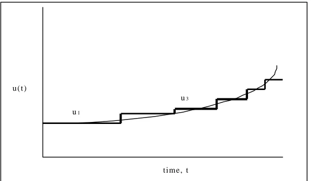
[image:2.612.144.460.540.724.2]As an example, Fig. 1 shows a piecewise constant approximation for a control profile with 6 intervals. Since two parameters are sufficient to describe the control profile in each interval, the entire control profile is defined by 12 parameters. These can then be added to any other decision variable in the optimization problem to form a finite set of decision variables. The optimal control problem is then solved using a nested procedure: the decision variables are set by an optimizer in an outer level and for a given instant of these variables, dynamic simulation is carried out to calculate the objective function and constraints as given from Eqns. (1) to (3). These outer problem is a standard nonlinear programming problem (NLP), solvable using a suitable method such as Sequential Quadratic Programming (SQP). Since the DAE’s are solved for each function evaluation, this has been called a feasible path approach.
Fig. 1: Piecewise Constant Discretization of Continuous Control Function u ( t )
u1
u3
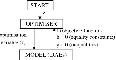
Fig. 2 illustrates a typical computation sequence for the solution of optimization problem presented by eqn. (3). The calculation sequence is started with an initial estimate of vector z. For each iteration (of the OPTIMIZER) dynamic optimization requires full integration of the model equations from t=[0,tF] to evaluate the objective function J
and the constraints (h and g) which are then passed to the OPTIMIZER. OPTIMIZER then takes a step in z and the process is repeated until convergence is achieved within an acceptable accuracy.
Fig. 2: Computational sequence of dynamic optimization problem
However, in many chemical processes, especially inherently dynamic batch process, it is not always possible to model actual processes. Therefore, the state predicted by using the model (eqn. 1) will be different than that of the actual process and will result in process-model mismatches. The implementation of the optimal operating policies obtained using the model will not result in a true optimal operation. Regardless of the nature of the mismatches, a true process can be described (Agarwal, 1996) as:
( ) ( ) ( )
( )
(
,
'
,
,
,
,
)
=
0
− −
−
t
x
t
u
t
v
e
t
x
t
f
x [t0,tF] (5)where
x
( )
t
− is the true set of all state variables,
x
−'
( )
t
denotes the derivatives
x
( )
t
− with respect to time;
v
−( )
t
isthe true set of time independent design variables;
e
x( )
t
isthe set of process-model mismatches for the state variables x; and the control vector
u
, and the functionf
are identical to those used in the model (eqn. 1). The error( )
t
e
x is in general time dependent and describes the entire deviation due to process-model mismatches.At any time t during the process operation, the true estimation of the state variables requires instantaneous values of the unknown mismatches
e
x( )
t
. To find theoptimal operation policies in terms of the decision variables z (Eqn 3) of a dynamic process using the model will require accurate estimation of
e
x( )
t
for each iteration on z duringrepetitive solution of the optimization problem. Although estimation of process-model mismatches for a fixed operation condition (i.e. for one set of z variables) can be
obtained easily, the prediction of mismatches over a wide range of operating conditions can be very difficult. In this case, the plant-model mismatch is estimated using neural networks and the optimization methodology mentioned above modified to cater for this mismatch estimation, which is described in the next section.
3.0 DYNAMIC PROCESS OPTIMIZATION WITH PROCESS MODEL MISMATCH ESTIMATION 3.1 Modeling of Dynamic Process-Model Mismatches As the mismatches of the sate variables of a dynamic system (i.e. instant distillate and reboiler compositions in batch distillation) are dynamic in behavior, they have to be treated as such, and not as static systems. Neural networks have been known to be able to approximate non-linear continuous functions with a high degree of accuracy (Cybenko, 1989; Hussain et al., 1995). In this work, neural network techniques are used to model process-model mismatches. This method is also suitable and appropriate in dealing with the estimation of these mismatches on-line, due to its fast implementation time. Although black box in nature, it has the ability to approximate any function mapping from system inputs to outputs, from known input-output data. It performs much less computation time in on-line applications than the other methods since the computer-intensive parts of the work, i.e. its training, are normally done off-line. The method of training the neural network to perform system identification, i.e. prediction of the mismatches at discrete-time intervals is called forward modeling, the details of which can be seen in other references [Hussain, 1996].
In this example, the reflux ratio is considered the only governing factor for the optimal operation, which can vary within reasonable physical bounds during the operation of the actual process and also during the solution of the dynamic optimization problem. Therefore, all dynamic mismatch models should be able to predict the mismatches accurately within the bounds of the reflux ratio. For different values of the reflux ratio over a feasible length of time (within which the minimum time lies) the process-model mismatches for the state variables are generated using the actual process data (as given by the detailed model) and simple model predictions.
The development of these neural network-based estimators also requires both the state variables (predicted by the model) and the mismatches at discrete points within the time interval. However in generating the state profiles, the variable multistep length is used for efficient integration of the model equations, which does not produce the states at fixed discrete-time intervals. Hence, the states at discrete time steps are obtained using linear interpolation technique. For example, if the instant distillate compositions predicted
by the models are
x
d,k andx
d,k+1at timet
kandt
k+1,J (objective function) h = 0 (equality constraints) g < 0 (inequalities)
z
OPTIMISER
MODEL (DAEs)
optimisation variable (z)
then at any discrete time
t
i, which lies within[
t
k,
t
k+1]
, the instant distillate composition( )
x
d,i is calculated using the following expression:(
i k)
dkk k
k d k d i
d
t
t
x
t
t
x
x
x
,1 , 1 ,
,
−
+
−
−
=
+ +
(6)
Usually, discrete points are of equal length (
∆
=
t
i+1−
t
i) which usually represents the sampling time of the actual process. In the absence of the actual process data, state variables for the actual process are predicted from the detailed model at discrete time interval using the same technique outlined above. For example, the instant distillate composition of the actual process at discrete timei
t
, is given byx
d,i−
. The discrete mismatch at
t
i willtherefore be
e
xd,i=
x
d,i−
x
d,i−
.
The approach we adopted here is to augment the neural network inputs with corresponding discrete present and past values of the state variables, the past values of the mismatches together with the relevant optimization variables (z) (e.g. reflux ratio in batch distillation). It is to be noted that we develop separate mismatch models for each state variable. The data are fed to the network in a moving window scheme. In this scheme, all the data are
moved forward at one discrete-time interval until all of them are fed into the network. The whole batch of data is fed into the network repeatedly until the training error criterion is achieved. The method of training the network is by the normal back propagation with momentum term as well as an adaptive learning rate to speed up the rate of the convergence.
3.2 Reformulation of Algorithm for Dynamic Process Optimization
The solution of dynamic optimization problem as presented by Eqn. (3) requires continuous profiles for the state variables for any given reflux ratio and therefore requires continuous profiles for the mismatches. However, the neural network mismatch estimator predicts the mismatches
[image:4.612.95.504.421.703.2]at discrete times,
t
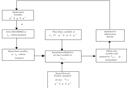
k as mentioned in the previous section. Hence, to obtain the state variables incorporating mismatches requires the estimation of all the state variables at these discrete times. For any reflux ratio and batch time (as determined by the OPTIMIZER, Fig. 2) this is achieved by integrating the model without adding mismatches. The estimated mismatches are then added to these state variables and these updated state variables values are then converted back into the continuous profile by the interpolation techniques above. They are then utilised within the optimizer routine and the whole procedure repeated for the next time step, as illustrated in Fig. 3. In this work the prediction of mismatch profiles starts from discrete point 3. Time t=0 represents discrete point 1 whereFig. 3: Incorporation of Model Mismatch in State Variable
Optimization Variables
u l
u u
u ≤ ≤
Solve DAE MODEL at
k
t without mismatch
Interpolation Method to get state variables at
1
+
k
t
Plant Data available at
k
t for u l ≤ u ≤ uu
Obtain state variables with mismatch at tk + 1 by
interpolation
u
Obtain State variables at tk without
mismatch
Implement in Optimization Routine
Neural Network Predicts mismatch
for any tk + 1 u l
u u
the mismatch is assumed to be zero for all the state variables. A discrete point 2, mismatches are initialized with a given value (obtained by judging the trend in all the data set used for the training of the neural network). In this work the length of the discrete time interval used is 15 minutes, (which is an acceptable sampling time for a batch distillation process).
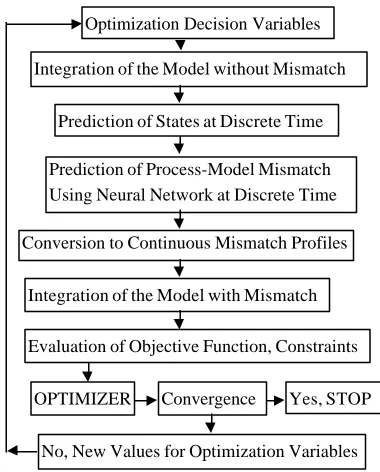
Fig. 4 illustrates the general optimization framework to obtain the optimal operation policies for dynamic processes with process-model mismatches as purposed in this work.
[image:5.612.397.478.392.473.2]In summary, the following steps are performed in this scheme: (1) Dynamic set of the process-model mismatches data is generated for different values of the optimization variables (z) covering the range within the process is to be operated optimally. These data are then used to train the net. Once trained, the net predicts the process-model mismatches for any sets of values of z as a function of time at discrete-time intervals. (2) During solution of the dynamic optimization problem, the model has to be integrated many times, each time using a different set of z. The process-model mismatches profiles at discrete-time intervals, which has been estimated by the neural network, are then added to the simple dynamic model during the optimization process. During this course of solving the dynamic model, these discrete process-model mismatches are converted to continuous function of time using linear interpolation technique so that they can be easily added to the model within the optimization routine. One of the important features of the framework is that it allows the use of discrete process data in a continuous model to predict discrete and/or continuous mismatch profile.
Fig. 4: Computational sequence for dynamic process optimization with process-model mismatch
4.0 CAS E STUDY: BATCH DISTILLATION PROCESS
[image:5.612.91.281.457.693.2]Batch distillation is an excellent representative example of a whole class of complex dynamic optimization problem (see Fig. 5). It represents an interesting field of academic and industrial research, for several reasons. Even for simple binary mixtures many alternative operations are possible. There is ample scope for optimization with complex trade-offs as a result of the many degrees of freedom available (Macchietto and Mujtaba, 1996). The accurate modeling of this process is difficult and can be very complex. Therefore, a simple model incorporated with process-model mismatches is very attractive for on-line prediction of states and also for finding optimal operation policies on-line or off-line. In the absence of real process data in the literature, we assume that a rigorous model based on the detailed mass and energy balances and rigorous thermophysical property calculations represent the actual batch distillation process. In this work, we have used the model used by Macchietto and Mujtaba (1996). The details of the model equations will not be presented here. However, it is to be noted that unlike the simple model the detailed model included plate holdup, which results to a large number of state variables (differential variables). At any given time, for a particular reflux ratio, the difference in predictions of the state variables by the two models of different complexity gives the process-model mismatches.
Fig. 5: Schematic of a batch distillation process
4.1 Optimal Operation without Process-Model Mismatch
Here, we considered a simple binary mixture. The separation task is defined as: recover 90% of component A (more volatile) as distillate product with purity of 0.95 molefraction in component A. The reflux ratio is chosen as the only control variable, which governs the performance of the process. The objective is to obtain reflux ratio policy which all achieve the separation task in minimum time. The column configuration and input data are given in Table 1.
Table 1: Column Configuration and Input Data
Number of Stages, N 12 No. of components, Nc 2 Initial feed, B0, kmol 10.0
Initial feed composition, xB0 <0.5, 0.5>
Condenser holdup, kmol 0.1 Vapour boilup rate, V, kmol/hr 5.0
LD
L V
Optimization Decision Variables
Integration of the Model without Mismatch
Integration of the Model with Mismatch Prediction of States at Discrete Time
Prediction of Process-Model Mismatch Using Neural Network at Discrete Time
Conversion to Continuous Mismatch Profiles
Evaluation of Objective Function, Constraints
OPTIMIZER Convergence Yes, STOP
The results at optimal solutions for both the actual model and the simple model are shown below.
Actual Process (Detail Model)
Optimum Reflux Ratio = 0.914
Minimum Time, hr = 10.99
Amount of Distillate, kmol = 4.74 No. of iteration for optimisation = 10
Model (Simple)
Optimum Reflux Ratio = 0.924
Minimum Time, hr = 12.51
Amount of Distillate, kmol = 4.74 No. of iteration for optimisation = 12
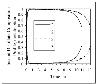
The instant distillate composition profiles for the actual process (detailed model) and that predicted by the model (simple model) are shown in Fig. 6. The simple model predicts significantly higher operation time (about 14%) compared to that by the actual process although the variation in the optimal reflux ratio is within 1%. The results clearly show the undesired effect of process-model mismatches on the optimal operation.
4.2 Optimal Operation with Process-Model Mismatch
Here we implement the general optimization framework with the incorporation of the process-model mismatches in the batch distillation study above. The separation task and the objective are same as those presented in Table 1. The optimization variables are the reflux ratio and the batch time.
The solutions of the optimization problem in this case are:
Optimization Reflux Ratio = 0.915
Minimum Time, hr = 11.09
Amount of Distillate, kmol = 4.74 No. of iteration for optimization = 7
The results in terms of reflux ratio and minimum batch time are sufficiently close to those of the actual process. At the optimal solution, the instant distillate composition profiles of the actual process and that obtained using model with process-model mismatches are presented in Fig. 7. These clearly show that the strategy was able to predict the dynamic mismatch profiles with sufficient accuracy and hence suitable to be used as the process-model mismatch predictor in any optimization framework.
0 0.1 0.2 0.3 0.4 0.5 0.6 0.7 0.8 0.9 1
0 1 3 4 5 6 8 9 10 11 12
Time, hr
Instant Distillate Composition
Profile, molefraction
2
2
3
[image:6.612.326.523.56.228.2]3
Fig. 6: Instant distillate composition profiles 2-Actual process
3-Simple model
0 0.2 0.4 0.6 0.8 1
0 1 3 4 5 6 8 9 10
Time, hr
Instant Distillate Composition
Profile, molefraction
1
1
2
2
Fig. 7: Instant Distillate Composition Profiles 1-With mismatch
2-Actual process
5.0 CONCLUSION
The optimization algorithm has been tested using a batch distillation process. For a given separation task the use of simple model for this process predicted about 14% higher optimal batch time compared to that of actual process (represented by a detailed model). This was due to the presence of substantial process-model mismatch. Inclusion of mismatches in the simple model allowed us to obtain optimal operation policy (in terms of reflux ratio and batch time) very close to that of the actual process. Application of the purposed technique to cases with more that one reflux ratio interval and to multi-component non-ideal systems are currently being investigated. This technique is also suitable for real on-line applications where process-model mismatch inherently exists at all times.
6.0 REFERENCES
[1] M. Agarwal, Batch Processing Systems Engineering: Fundamentals and Applications for Chemical Engineering, G.V. Reklaitis et al. eds., Series F: Computer and Systems Sciences, Springer Verlag, Berlin, 143, 295, 1996.
[2] J. E. Cuthrell, and L. T. Biegler, Comput. Chem. Engng. 13 (1/2), 49, 1989.
[3] G. Cybenko, Math. Cont. Sig. Syst. 2, 303, 1989.
[4] S. Farhat, M. Czernicki, L. Pibouleau, and S. Domenech, AIChE J. 36(9), 1349, 1990.
[5] M. A. Hussain, PhD Thesis, Imperial College, London, 1996.
[6] M. A. Hussain, J. C. Allwright, and L. S. Kershenbaum, (1995), Proceedings of IChemE -Advances in Process Control 4, York, 27-28 September, p. 195, 1995.
[7] J. S. Logsdon, U. M. Diwekar, and L. T. Biegler, Trans IChemE, 68, Part A:434, 1990.
[8] K. R. Morison, PhD Thesis, Imperial College, London, 1984.
[9] I. M. Mujtaba, and S. Macchietto, J. Proc. Cont. 6 (1), 27, 1996.
[10] S. Macchietto, and I. M. Mujtaba, Batch Processing Systems Engineering: Fundamentals and Applications for Chemical Engineering, G. V. Reklaitis et al. eds., Series F: Computer and Systems Sciences, Springer Verlag, Berlin, Vol. 143, 174, 1996.
[11] V. S. Vassiliadis, R. W. H. Sargent, and C. C. Pantelides, IEC Res., 33 (9), 2123, 1994.
[12] S. Walsh, I. M. Mujtaba, and S. Macchietto, Acta chimica Slovenica. 42 (1), 69., 1995.
BIOGRAPHY
Iqbal Mujtaba obtained his doctorate at Imperial College, London in 1989. He is now a senior lecturer at the department of Chemical Engineering, University of Bradford, U.K. His research areas include optimisation, control and computer-aided process engineering and has published many papers in international journals in these area.