ENSEMBLE SELECTION AND OPTIMIZATION BASED ON SOFT SET THEORY FOR CUSTOMER CHURN CLASSIFICATION

ISSN: 1992-8645 www.jatit.org E-ISSN: 1817-3195

121

OPTIMAL FEATURE SELECTION FOR CLASSIFICATION OF

ELECTRICITY CONSUMPTION

1_{ZUHAINA ZAKARIA}

, 2NOORITAWATI MD TAHIR

1,2

Faculty of Electrical Engineering, Universiti Teknologi MARA (UiTM) 40450, Shah Alam, Selangor, Malaysia

1

[email protected], [email protected]

ABSTRACT

Feature selection is the essential process to obtain the best feature vectors in pattern recognition system. These feature vectors contain information describing the original data’s important characteristics. In this research, a framework based on factor analysis technique namely the Principal Component Analysis (PCA) is performed to determine the best features extracted from the daily load curve prior to clustering process. The rules of thumb applied include Bartlett’s test of sphericity, Kaiser-Meyer-Olkin (KMO) measure, Kaiser Criterion, Scree test along with Varimax approach. Accordingly, KMO as well as Bartlett’s test suggested the data factorability is significant. Furthermore, Kaiser Criterion and Scree test together with component matrix approach implied that the first two most significant factor must be retained whilst Varimax approach confirmed that clustering analysis should comprise of the entire load curve values. Upon selection of features, the capability of fuzzy clustering in classifying these features attained from 247 feeders in a particular distribution network is examined. Initial results demonstrated the effectiveness of feature selection process and the potential of fuzzy clustering in particular the fuzzy c- means (FCM) in classifying electrical energy consumption.

Keywords: Feature Selection, Load profiling, clustering, fuzzy relation, Principal Component Analysis

1. INTRODUCTION

The use of pattern recognition (PR) and classification is fundamental to many applications such as remote sensing, computer vision, artificial intelligence and medicine. There are three main aspects involved in designing a PR system which includes preprocessing of the raw data, feature extraction and classification. Among the three aspects, feature extraction and selection is the key process and require special attention. Feature selection is a process to select a subset of relevant features which performs best in the process of classification. In many cases, this procedure resulted better classification and also reduce the cost of classification by reducing the number of features that need to be collected [1].

In electricity industries, metering and billing systems has been affected by the price of energy and these have changed the electricity deregulation scenario. In many countries, electricity consumers do not have to rely on a single electricity provider since there are many competitive electricity providers. Consequently, electric utilities companies need to fully equip themselves with suitable tariff formulation and enhanced their marketing strategies [2-5]. For instance, analyzing

consumer behavior in using electricity is necessary to understand their required demand. Although the monthly billing data could provide the demand characteristic but sometimes it is inadequate. A more accurate approach is to install interval meter either quarterly-hourly, half-hourly or hourly at each appropriate points for analyzing the electricity demands. However, this method is expensive in terms of equipment, maintenance and processing [6].

Another cost-effective approach is to acquire consumers’ load profile by classifying the load curves. Efforts toward determining load profiles by categorizing consumers have been performed and reported in several articles. The regulatory authorities in United Kingdom regulatory have established two generic profiles for domestic and six for non-domestic consumers to represent their 100 kW demand category consumers [7].

ISSN: 1992-8645 www.jatit.org E-ISSN: 1817-3195

122 flexible in selecting the cluster boundary. Thus, and FCM was chosen as the clustering algorithm in this work.

However, to obtain a better clustering, the most valuable subset of the original features must be used as the input to the clustering process. At a glance, it may seem that certain particular features are important such as number of peaks in the load curve, the time of the peaks or area under the curve. However, work in [16] argued that some other subtler features of load curve will also provide important indication of the energy-usage pattern. In their work, they stated that the whole load curve should be considered. To confirm this theory, the entire daily load curve is used in this work and analysed using Principal Component Analysis (PCA) before it is used as an input to FCM. In this paper, section 2 explains the proposed algorithm employed followed by description of experimentation and results in section 3. Finally, conclusion of the study is presented in section 4.

2. METHODOLOGY

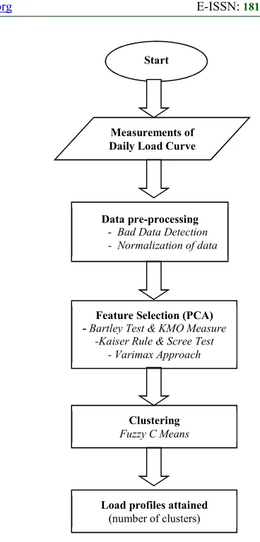
An overview of the proposed method that outlines the whole process is shown in Figure 1. Daily load curves were recorded for every 30 minutes and were used as input to the clustering analysis. Thus, there were 48load values in a 24-hour load curve. Only weekday load curves are considered in this study.

The pre-processing stage is essential for detection of missing or unusual data and normalization of data before the clustering process. In this study the recorded data was in kilowatt (kw), thus normalization into per unit values are required. The suitable normalizing factor is either the average power over a certain time period [17] or the peak power [18]. The peak power of the whole measurement was chosen as the normalizing factor in this work. After the pre-processing stage, the data is prepared for the feature selection process as described in section 2.1. The best features of the data will be used in the clustering process as discussed in section 2.2.

2.1 Principal Component Analysis (PCA)

The main application of PCA is to reduce the number of variables and to detect structure in the relationships between variables. There are three main steps in conducting factor analysis in PCA and each of the steps is explained in the next subsections.

2.1.1 Assessment of data suitability for factor analysis

In order to determine the strength of the relationship among the variables, the correlation matrix need to be inspected for coefficients greater than 0.3. Two statistical measures, Bartlett’s test of sphericity and the Kaiser-Meyer-Olkin (KMO) Measures can be used to help assess the factorability of the data [19].

Bartlett’s test of Sphericity examines the hypothesis that the correlation matrix is an identity by looking at the significance level. For a very small values that is less than 0.05, indicates that there are probably significant relationships among the variables. However, if the value of the test statistic for Sphericity is large and the associated significant level is small, the population correlation matrix is not an identity matrix. On the other hand, the Kaiser-Meyer-Olkin statistic (KMO) is an index

Figure 1: Overview of the overall system

Load profiles attained

(number of clusters)

Clustering Fuzzy C Means Feature Selection (PCA) - Bartley Test & KMO Measure

-Kaiser Rule & Scree Test - Varimax Approach

Start

Measurements of Daily Load Curve

Data pre-processing

- Bad Data Detection

ISSN: 1992-8645 www.jatit.org E-ISSN: 1817-3195

123 for comparing the magnitudes of the observed correlation coefficients to the partial correlation coefficients. The KMO index ranges from 0 to 1, with 0.50 considered suitable for factor analysis [19-20]

2.1.2 Factor extraction

This step will determine the least number of factors that significantly indicates the inter-relations among the set of variables. Two techniques can be utilized to assist for decision making namely the Kaiser’s criterion and Scree test. The Kaiser’s criterion states that it is not worth retaining any eigenvalue with a variance of less than one because it contains less information than the original variables. Thus, the Kaiser rule only retains eigenvalues that are greater than or equal 1. However, this rule usually retains too many eigenvalues for large variable spaces p [21].

The second technique, Catell’s Scree test observes the plot of the eigenvalues against the factor number k. This will involve a certain degree of subjectivity since there is no formal numerical cut-off based on the eigenvalues. The main idea behind this test is that important factors have a large eigenvalue and as such explain a large part of the total variance. If the eigenvalues are plotted, they form a curve heading towards almost 0% variance explained by the last dimension. Thus, the point at which the curve levels-out, sometimes referred to as the ‘elbow’ indicates the number of useful eigenvalues, which are present in the data [21].

2.1.3 Factor rotation and interpretation

The number of factors which determined need to be interpreted and one way of doing this is by factors rotation. Rotation maximizes and minimize high item and low item loadings respectively, therefore producing a more interpretable and simplified solution. There are many different rotational techniques and the most commonly used is the Varimax method and will be employed in this work.

2.2 Fuzzy C-Means (FCM)

Generally, classical algorithm of cluster analysis is hard partitioning which means each object belongs to only one cluster but soft partitioning is required for objects which have vague attributes. Application of soft partitioning using fuzzy set theory were proposed in [22] and [23]. FCM which is based on objective function is developed to

improve previous clustering approach [24]. FCM will classify each data point into a cluster based on degree of membership grade. This is achieved by minimizing the following objective function:

2

1 1

N C m

m ij i j

i j

J

u

x

c

= =

=

∑ ∑

−

where C is the number of cluster, N is the number of load profile, m is a weighting parameter, in general m=2, uij is the degree of membership of xi

in the cluster j, xi is the profile of ith feeder of

measured data, cj is the jth center of the cluster, and ||*|| is any norm expressing the similarity between any measured data and the center. The value of C for the data needs to be identified if it is unknown. The weighting parameter m controls the fuzziness in the clustering process. This value is normally chosen heuristically but researches has found that best value of m in the interval of 1.5 - 2.5 [25]. However, many users of FCM prefer the interval midpoint, m=2.

FCM begins with guessing the cluster centers which is most likely incorrect. Next, every data point is assigned a membership grade to each cluster. The cluster centers and the membership grades for each data point will be updated iteratively until the cluster centers move to the right location within a data set. FCM will produce the final membership matrix U and cluster centers. A data point which has maximum membership grade will then be assigned into a particular cluster.

2.3 Cluster Validity

Although, the number of clusters will be discovered naturally since clustering algorithms is an unsupervised process however, the final partition of the data need to be evaluated. This procedure is called cluster validity and it is use to determine the optimal number of clusters in a data set. Many different indices for cluster validity have been developed [20]. In this study, four widely used indices i.e. nonfuzziness index (NFI) [26, 27], minimum hard tendency (MinHT), mean hard tendency (MeanHT) [28] and separation index (SI) [29] will be employed.

3. RESULTS AND DISCUSSION

ISSN: 1992-8645 www.jatit.org E-ISSN: 1817-3195

124 every half-hour, totaling of 48 values for each feeder.

3.1 Results from PCA

This section discussed the results from factor analysis procedure which were performed using the statistical software, SPSS. The results from the KMO measures and Bartlett’s test are as tabulated in Table 1. The KMO value obtained is 0.963 and that indicated a good factor analysis value. Next, three values were calculated from the Bartlett’s test namely the approximate chi-square, degree of freedom (df) and significant value (sig). However, only the Sig. value is considered and it should be 0.05 or lower. The Bartlett’s test attained in this case study is 0.000, which indicates as ‘significant’. Thus, factor analysis is apt for this data.

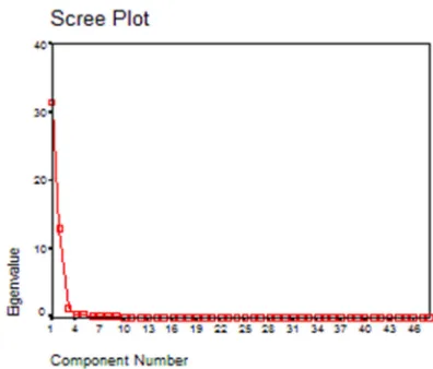
Further, Kaiser’s criterion is used for extraction of factors and merely components with eigenvalue of 1 or more are to be considered. As illustrated in Table 2, it is observed that only the first three components specifically 31.517, 13.156, and 1.275 owned an eigenvalue of above 1. (Note that only the first 5 components are revealed due to lack of space.). Generally, the Scree plot is more accurate than Kaiser’s criterion [21].

Therefore, the Scree plot will also be examined to seek changes (elbow) in the plot and only components above these changes will be retained. As depicts in Figure 2, it is observed that component 1 and component 2 captured most of the variance in contrast to the remaining component. In addition, a distinct break is also examined between

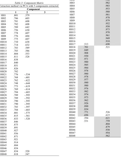
the second and the third component. Therefore, in our case, only the first two factors will be retained. Another way to verify the inference from the Scree plot is from Component Matrix which should indicate the loadings of each item in the three components that obtained eigenvalue of above 1.

However, as shown in Table 3, only component 1 & 2 are loaded with all items but none on component 3. Hence, this finding supports the earlier conclusion to retain only two factors. This demonstrated that results of factor extraction that are unaccompanied by rotation are likely difficult to be interpreted regardless of which method of extraction used. Thus, the next step is to rotate these two factors for ease of interpretation. For this data sample, Varimax rotation technique is adopted since easier and clearer interpretation can be accomplished.

Table 4 illustrated the loadings of each variable on the two selected factors according to Rotated Component Matrix. The shaded area illustrated that the main loadings on Component 1 are from HH18 until HH41 whilst the main loadings on Component 2 are from HH1 until HH17 as well as from HH42 until HH48. Although both components are loaded with variables at HH17, HH40, HH41, HH42 and HH43, only high loadings are considered. The remaining variables loaded sturdily on only one component with both This revealed a simple structure meaning that there are only two main patterns in the data.

Additionally, Table 5 detailed the two-factor solution that a total of 93% of the variance with Component 1 contributing 46.7% and Component 2

Table 1: Kaiser-Meyer-Olkin Statistic and Bartlett's Test

Kaiser-Meyer-Olkin

Measurement of Sampling Adequacy

0.963

Bartlett's Test of Sphericity

Approx. Chi-Square 42365.364

df 1128

Sig. 0.000

Table 2: Detail values of total variance

Initial Eigenvalues

Comp Total % of Variance Cum %

1 31.517 65.661 65.661

2 13.156 27.408 93.070

3 1.275 2.656 95.726

4 0.510 1.063 96.789

5 0.432 0.899 97.688

ISSN: 1992-8645 www.jatit.org E-ISSN: 1817-3195

125 contributing 46.3%. The interpretation of these two components is consistent since the variables in Component 1 are for time period from 8 am until 8 pm. Alternatively, the time period for variables in Component 2 are vice versa. Thus, these show that all values are vital and proven that the entire load curve values are significant and must be contained in the clustering analysis.

Table 3: Component Matrix

Extraction method via PCA with 3 components extracted.

Component

1 2 3

HH1 .801 .579

HH2 .786 .603

HH3 .781 .608

HH4 .782 .608

HH5 .709 .642

HH6 .756 .630

HH7 .778 .607

HH8 .776 .604

HH9 .775 .607

HH10 .710 .638

HH11 .714 .632

HH12 .783 .589

HH13 .783 .586

HH14 .804 .553

HH15 .811 .528

HH16 .838

HH17 .840

HH18 .851

HH19 .826

HH20 .782

HH21 .776 -.534

HH22 .768 -.601

HH23 .762 -.622

HH24 .748 -.644

HH25 .773 -.619

HH26 .769 -.614

HH27 .784 -.603

HH28 .789 -.595

HH29 .789 -.592

HH30 .790 -.595

HH31 .790 -.595

HH32 .783 -.597

HH33 .784 -.603

HH34 .801 -.575

HH35 .815 -.561

HH36 .833 -.528

HH37 .846

HH38 .875

HH39 .891

HH40 .927

HH41 .936

HH42 .871

HH43 .921

HH44 .914

HH45 .884

HH46 .854

HH47 .834 .520

HH48 .818 .547

Table 4: Rotated Component Matrix

Extraction method via PCA and analysis rotation method using Varimax along with Kaiser Normalization.

Component

1 2

HH1 .975

HH2 .982

HH3 .982

HH4 .983

HH5 .953

HH6 .980

HH7 .981

HH8 .978

HH9 .979

HH10 .952

HH11 .950

HH12 .973

HH13 .970

HH14 .961

HH15 .949

HH16 .910

HH17 .513 .690

HH18 .701 .521

HH19 .849

HH20 .908

HH21 .930

HH22 .971

HH23 .980

HH24 .985

HH25 .984

HH26 .978

HH27 .980

HH28 .978

HH29 .977

HH30 .980

HH31 .980

HH32 .976

HH33 .982

HH34 .974

HH35 .973

HH36 .962

HH37 .926

HH38 .890

HH39 .834

HH40 .771 .526

HH41 .696 .615

HH42 .594 .621

HH43 .531 .759

HH44 .804

HH45 .879

HH46 .930

HH47 .954

ISSN: 1992-8645 www.jatit.org E-ISSN: 1817-3195

126 3.2 Results from FCM

Since FCM is an supervised clustering algorithm, the maximum number of clusters, C needs to be determined. Although there are only three main categories of consumers connected to the feeders, C = 5 is chosen to give some flexibility to the clustering process. Therefore, the clustering algorithm was repeated from the minimum C= 2 until C = 5. For each values of C, cluster validity index computed as shown in Table 6. Index value for S is at minimum values while indices of NFI, MinHT and MeanHT should be at maximum values to determine the optimal number of clusters.

Based on the results in Table 6, the optimal number of clusters could be C = 3 or 4. However, since all parameters in cluster 3 fit these criteria aside from MinHT, C = 3 is chosen as the optimal number of clusters. Each cluster now has several numbers of feeders in it and by determining the average of the load diagrams, a typical load profile (TLP) for each cluster can be determined.

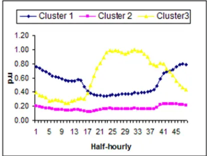
TLP for each cluster which representing three main categories depicted in Figure 3. From the results, a few salient characteristics have been discovered and outlined below.

i) TLP for cluster 1 shows the curve gradually decrease from 12 midnight and the load drastically increase in load between half-hour 14 – 15 (6.30 am – 7.00 am) and decreasing again from half-hour 16 – 20 (around 7.30 am – 9.30 am). For the rest of the day, the load is increasing slightly with small peaks during mid-day. Later, the load gradually increases from half-hour 40 onwards (7 pm).

ii) On the contrary, TLP for cluster 2 does not show any notable pattern. The load is quite flat with small peaks for the entire day. The TLP also shows very low load value compared with the other TLP. This shows that the clustering process succeeded in identifying the differences between the macro categories. iii) The pattern of TLP for cluster 3 gradually

increases from early morning and significantly increases from half-hour 16 (approximately 7.00 am). The curve reached its peak at 12 noon and 3 pm. There is a sharp decrease between these two peaks. Then, it gradually decreases again with small peak at about 8 pm.

From the above description and also since the feeders’ category of consumers are made known earlier, each TLP can be compared to a specific type of consumer for validation purposes.

Table 5: Detail values of total variance

Initial Eigenvalues

Component Total % of Variance

Cumulative %

1 31.517 65.661 65.661

2 13.156 27.408 93.070

3 1.275 2.656 95.726

4 0.510 1.063 96.789

5 0.432 0.899 97.688

Rotation Sums of Squared Loadings

Total

% of Variance

Cumulative %

22.421 46.71 46.71

22.22 46.291 93.001

1.308 2.725 95.726

Table 6: Calculation of Cluster Validity Indices for C=2 until C=5

Cluster 2 3 4 5

NFI 0.465 0.5439 0.509 0.4924

MinHT 0.7272 0.7519 0.8578 0.831

MeanHT 0.5842 0.6392 0.6209 0.5523

S 0.2288 0.1265 0.1891 0.2632

ISSN: 1992-8645 www.jatit.org E-ISSN: 1817-3195

127

As seen in Figure 4 through Figure 6, typical load profile for cluster 1, 2 and 3 are compared with random load curve that represents the electricity consumption for domestic, commercial, and small-scale industries respectively. Each typical load profile fit the pattern of the categories as clearly shown from these figures. The findings indicated that FCM is capable to cluster the feeders into main categories distinctly.

4. CONCLUSION

In conclusion, this study has presented a framework of feature selection method based on PCA. Experimental results stated that factorability of data is achieved via KMO and Bartlett Test. Both Kaiser Rule and Scree test are proven relevant for optimal feature selection process. In addition, the Varimax rotation technique verified the theory that the entire daily load curve values are vital for clustering purpose.

Further testing performed using 247 daily load curves from distribution feeders suggested that the data can be clustered optimally into 3 clusters. Averaging the load curves in each cluster established a typical load profiles which also fitted each cluster accordingly. Results attained confirmed that the process of feature selection together with fuzzy clustering specifically FCM has successfully classified electricity demand according to its pattern.

ACKNOWLEDGMENT

This work was supported by Fundamental Research Grant Scheme (FRGS) No: 600-RMI/FRGS 5/3 (143/2015) awarded by Ministry of Higher Education (MOHE) Malaysia. The authors also thanked Institute of Research Management and Innovation (IRMI), Universiti Teknologi MARA (UiTM), Shah Alam, Selangor, Malaysia for the support given in this research.

REFERENCES:

[1] A. K. Jain, R.P.W. Duin, and J. Mao, “Statistical Pattern Recognition: A Review”, in Proceeding of EEE Transactions on Pattern Analysis and Machine Intelligence, 22, (1), 2000.

[2] B. Stephen, A. J. Mutanen, S. Galloway, G. Burt and P. Jarventausta, "Enhanced Load Profiling for Residential Network Customers," in IEEE Transactions on Power Delivery, vol. 29, no. 1, pp. 88-96, Feb. 2014.

Fig 4: Comparison of TLP for Cluster 1 with daily load curve for domestic consumer

Fig 5: Comparison of TLP for Cluster 2 with daily load curve for commercial consumer

ISSN: 1992-8645 www.jatit.org E-ISSN: 1817-3195

128 [3] M. Piao, H. S. Shon, J. Y. Lee and K. H. Ryu,

"Subspace Projection Method Based Clustering Analysis in Load Profiling," in

IEEE Transactions on Power Systems, vol. 29,

no. 6, pp. 2628-2635, Nov. 2014.

[4] D. Colley, N. Mahmoudi, D. Eghbal and T. K. Saha, "Queensland load profiling by using clustering techniques," Power Engineering Conference (AUPEC), 2014 Australasian Universities, Perth, 2014, pp. 1-6.

[5] G. Zhou, W. Zhao, X. Lv, F. Jin and W. Yin, "A novel load profiling method for detecting abnormalities of electricity customer," PES General Meeting | Conference & Exposition, 2014 IEEE, National Harbor, MD, 2014, pp. 1-5.

[6] D. Gerbec, S. Gasperic, F. Gubina, "Determination and allocation of typical load profiles to the eligible consumers," Power Tech Conference Proceedings, 2003 IEEE Bologna , vol. 1, pp.5, 2003.

[7] S. V. Allera and A. G. Horsburgh, "Load Profling for Energy Trading and Settlements in the UK Electricity Markets," presented at DistribuTECH Europe DA/DSM Conference, London, 1998.

[8] T. Marijanic, D. Karavidovic, "Load profiling in an opening electricity market," AFRICON 2007, pp.1-5, 2007.

[9] A. Mutanen, M. Ruska, S. Repo, P. Jarventausta, "Customer Classification and Load Profiling Method for Distribution Systems," IEEE Transactions on Power Delivery, vol.26, no.3, pp.1755-1763, 2011. [10]I. B. Sanchez, I. D. Espinos, S. Moreno, L.

Quijano, I. N. Burgos, "Clients segmentation according to their domestic energy consumption by the use of self-organizing maps," Energy Market, 2009. EEM 2009. 6th International Conference on the European, pp.1-6, 2009.

[11]W. Yuan-Kang, "Short-term forecasting for distribution feeder loads with consumer classification and weather dependent regression," Power Tech, 2007 IEEE Lausanne, pp. 689-694, 2007.

[12]S. Ramos, Z. Vale, "Data Mining techniques to support the classification of MV electricity customers, " 2008 IEEE Power and Energy Society General Meeting - Conversion and Delivery of Electrical Energy in the 21st Century, pp.1-7, 2008.

[13]Lo, K. L., Zuhaina Zakaria, and C. S. Ozveren. “Fuzzy Classification and Statistical Methods for Load Profiling: A Comparison.” In

International Conference on Advances in Power System Control, Operation and

Management, 2003.

[14]Lo, K. L., and Zuhaina Zakaria. “Electricity Consumer Classification Using Artificial Intelligence.” In Universities Power Engineering Conference, 2004. UPEC 2004. 39th International, 1:443–47 Vol. 1. IEEE, 2004.

[15]Zakaria, Z., M. N. Othman, and M. H. Sohod. “Consumer Load Profiling Using Fuzzy Clustering and Statistical Approach.” In Research and Development, 2006. SCOReD 2006. 4th Student Conference on, 270–74. IEEE, 2006.

[16]J. A. Jardini, "Daily Load Profile for Residential, Commercial and Industrial Low Voltage Consumers," IEEE Transaction on Power Delivery, vol. Vol.15, pp. 375-380, 2000.

[17][7] G. Chicco, R. Napoli, F. Piglione, P. Postolache, M. Scutariu, and C. Toader, "A Review of Concepts and Techniques for Emergent Customer Categorisation," presented at TELMARK Discussion Forum European Electricity Markets, London, 2002.

[18]A.G Riddel and K Manson, "Parameterisation of Domestic Load Profiles," Applied Energy, vol. 54, pp. 199-210, 1996.

[19]Tabachnick BG, Fidell LS. Using Multivariate Statistics. Boston: Pearson Education Inc; 2007.

[20]Hair J, Anderson RE, Tatham RL, Black WC. Multivariate data analysis. 4th Ed. New Jersey: Prentice-Hall Inc; 1995.

[21]IT Joliffe. Principal Component Analysis, Springer Series, 2000

[22]Journal of Math Analysis and Applications, vol. 13, pp. 1-7, 1966.

[23]R. Bellman, R. Kalaba, and L. Zadeh, "Abstraction and Pattern Classification," [24]M.-S. Yang, "A Survey of Fuzzy Clustering,"

Math. Compute. Modelling, vol. 18, pp. 1-6, 1993.

[25]L. Zadeh, "Similarity relations and fuzzy orderings," Information Sciences, vol. 3, pp. 177-200, 1971.

[26]N. R. Pal and J. C. Bezdek, "On cluster validity for the fuzzy c-means model," Fuzzy Systems, IEEE Transactions on, vol. 3, pp. 370-379, 1995.

ISSN: 1992-8645 www.jatit.org E-ISSN: 1817-3195

129 Conference on Fuzzy Systems, Seoul, Korea, 1996.

[28]M. Roubens, "Fuzzy clustering algorithms and their cluster validity," European Journal of Operational Research, vol. 10, pp. 294-301, 1982.