Full Length Research Article
POWER ELECTRONICS CONVERTERS FOR GRID INTREGRATED VARIABLE SPEED WIND
TURBINE
*Gaurav Singh Bhandari and Dr. M. Kowsalya
School of Electrical Engineering, VIT University, Vellore, India
ARTICLE INFO ABSTRACT
This paper represents dynamic modeling and simulation of variable speed wind turbine (VSWT) with grid and without grid connection using MATLAB/SIMULINK, a widely used power system analysis and dynamic tool. The variable speed wind turbine with single fed induction generator (IG) and power electronic converter, controller is modeled for dynamic analysis. Component model and equations are represented and implemented in MATLAB/SIMULINK. Controllable power inverter strategy is applied for capturing maximum power under varying speed of wind turbine and controlled reactive power for voltage regulation. Simulation studies give control performance analysis of a gearless VSWT under varying wind speeds.
Copyright © 2014. Gaurav Singh Bhandari and Dr. M. Kowsalya. This is an open access article distributed under the Creative Commons Attribution License, which permits unrestricted use, distribution, and reproduction in any medium, provided the original work is properly cited.
INTRODUCTION
Renewable energy sources is widely used in industry for avoid pollution and economic purpose. Solar energy is used for power generation with solar rays, hydro energy is used for power generation using water’s hydrostatic energy, wind energy is used for power generation using wind. Mostly wind energy is used for power generation purpose in comparison with hydro and solar energy due to following reasons. Wind farm setup require small geographical area in comparison with hydro energy due to setup hydro power plant that effects in human’s life, commercial user, residential area etc. wind energy can be obtained in day and night in comparison with solar energy because solar energy is obtained in only day if continuous rainy season occurs then solar energy is not possible for power generation purpose so power generation using wind energy is more comparison to solar energy. In this paper wind energy is modeled for power generation and torque is generated using wind turbine is given to Induction Generator (IG) that dives generator and controlled by using rectifier and inverter so that reactive power is controlled to avoid losses and improves power quality (Seul-Ki Kim and Eung-Sang Kim, 2007; Slootweg et al., 2003). Variable speed operation yields 20 to 30 percent energy than the fixed speed operation, reduces power fluctuations and improves reactive
*Corresponding author: Gaurav Singh Bhandari
School of Electrical Engineering, VIT University, Vellore, India
power supply. Falling prices of the power electronics have made the variable speed technology more economical and common. The distributed generation cannot connect easily to the electric power network without conducting evaluations on control performance and grid impact. Stable grid interface requires a reliable tool for simulating and assessing the dynamics of a grid connected variable speed wind turbine.
MATLAB/SIMULINK is a standard simulation tool for studying the behavior of electrical networks. Its graphic-based user interface allows the user to graphically assemble the circuit, run the simulation, analyze the results, and manage the data in a completely integrated graphical environment. The purpose of this paper is to provide simulation and dynamic performance and grid impact analysis capability of a gearless VSWT based on MATLAB/SIMULINK. The schematic diagram of the wind generation model is shown in Fig.1. The model system is composed of a fixed-pitch stall regulated wind turbine, a gearless direct drive generator and a controllable power electronics system, which consists of a simple diode rectifier and a six-IGBT voltage source inverter (VSI). A graphic-based model suitable for electromagnetic transient studies has been proposed based on mathematical equations. Model representation is shown in Fig.2. The aim of this paper is to design and simulate a open loop renewable energy source (wind) integrated with the grid.
ISSN:
2230-9926
International Journal of Development ResearchVol. 4, Issue, 3, pp. 592-598, March,2014
DEVELOPMENT RESEARCH
Article History:
Received 08th
January, 2014 Received in revised form 11th February, 2014 Accepted 15th February, 2014 Published online 14th March, 2014
Key words:
Gearless variable speed wind turbine (VSWT), Power electronics control,
Fig.1. Schematic Representation of gearless VSWT
Fig.2. Components proposed of simulation model
Matlab Simulink Based Modelling
Fig. 2 presents the proposed simulation model which consists of following components.
(1): Wind speed model for generating wind speed that can be applied to the rotor.
(2): Wind turbine for converting the kinetic energy contained in wind that can be applied to the generator.
(3): Model of generator and converter for converting mechanical power into electric power and determining the rotor speed.
(4): All components is connected to grid. Design is proposed in (Slootweg et al., 2003; Narayan Prasad Gupta et al., 2012).
Wind Speed Model
Wind speed is a combination of four component, gust speed, ramp speed, base speed, noise speed. Design of wind speed is proposed in (Anderson and Anjan Bose, 1983).
VWind = VGust + VRamp + VBase + VNoise
Gust Speed
Gust speed is sudden change in wind speed. it is given as:
VGust =
0 <
< < +
0 > +
(1)
VCOS = (MAXG/2){1-cos2 [(t/T1G) – (T1G/TG)]} (2)
TG = Gust Period in sec, T1G = Gust starting time in sec. MAXG = Gust peak in mi/sec, t = Time in sec. Ramp Speed Ramp speed is continuous varies with time. it is given : VRamp = 0 < 0 > < (3)
VRamp = MAXR[1 – (t-T2R)/(T1R – T2R)]m/sec (4)
T1R = Ramp starting time(s), T2R = Max time(s). Base Speed Base speed is constant speed. It is given as: VBase = KB where KB is constant Noise Speed Noise speed is continuous triangular wave or random variable with time. it is given as: VNoise = 2 ∑ [S (ωi)∆ω]1/2 Cos(ωi t + ɸi), t<0 (5)
Where ωi = (I – 1/2)∆ω, ɸi = a random variable on time interval o to2 . Sv (ωi)= (2KNF2|ωi|) ÷ ( 2[1 + (Fωi/µ )2]4/3) (6)
Where KN = Surface drag coefficient (0.004) F = Turbulane scale (2000), µ = Mean wind speed at reference height Wind Turbine Design Mechanical power extracted from Wind (Pm): Pm = Cp(ג, β)(PW) (7)
PW = 0.5ρAV3w (8)
ג(Tip speed)= (RBlade.ωr/Vw) (9)
Tm (Mechanical Torque) = (Pm/ωr). (10)
Cp(ג, β)is given by C1(C2 – C3β – C4β2 – C5)e-C6 + C7ג. (11)
Value of power coefficient from C1 to C7 are as follows: C1 = 0.5, C2 = 116/גi, C3 = 0.4, C4 = 0, C5 = 5, C6 = 21/גi, C7 = 0.0068. (1/גi)= (1/ג+0.08β) – (0.035/β3+1) (12)
Table 1. Parameter for wind turbine
Pm Mechanical power extracted from wind(W)
PW Kinetic energy contained in wind
Cp(ג,β) Power coefficient of Turbine
ρ Air density(kg/m3)=0.55kg/m3
A( R2
) Turbine swept area(m2
) R Turbine Radius(m) = 36.5m
ג Tip speed ratio of the rotor blade tip speed to wind speed
Vw Wind Speed(m/s)
Nominal wind speed =12.35m/s
ωr Generator Speed(RPM)
Generator base speed= 18 rpm Rating of wind turbine 2 MW
Design of Induction Generator
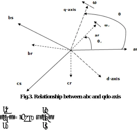
Single fed induction generator is used for power generation purpose because it is very economical and low cost. The two common reference frames used in the analysis of induction machine are the stationary and synchronously rotating reference frames. Each has its own advantage for some purpose. In the stationary rotating reference, the dq variables of the machine are in the same frame as those normally used for the supply network. It is convenient choice of frame when supply network is large or complex design is proposed in (Narayan Prasad Gupta et al., 2012; Yuya Izumi et al., 2011; Anderson and Anjan Bose, 1983). In the synchronously rotating reference frame, the dq variable are steady in steady state, a prerequisite when deriving the small-signal model about a chosen operating point. The Relationship between abc and qdo quantities of a reference frame rotating at an angular
speed ω, as shown in Fig 3. The transformation equation from
[image:3.612.65.287.269.481.2]abc to this qdo reference frame is given by:
Fig.3. Relationship between abc and qdo axis
0
= 0
Where the variable can be phase voltage, current, or flux linkage of the machine.
From Fig 3
θ (t) = ∫ ( ) + (0)Where ω(t) is speed of reference
frame.
(t) = ∫ (t) + (0) Where (t) is speed of rotor
0 =
⎣ ⎢ ⎢ ⎢
⎡ cos ( − ) cos ( + )
sin ( − ) sin ( + )
⎦ ⎥ ⎥ ⎥ ⎤ (13)
and its inverse is given by:
[Tqd0] -1
=
1
cos ( − ) sin ( − ) 1
cos ( + ) sin ( + ) 1
(14)
The stationary reference frame is used so speed of reference
frame (ω) = 0 and θ = 0.
Next transformation of stator phase voltage to qd0 stationary
voltage by θ = 0.
Step 1: vsq = vas - vbs - vcs , v s
d = √ (vcs - vbs) ,
v0 = (vas + vbs + vcs) (15)
Step 2: Transformation of rotor phase voltage to qd0
stationary voltage.
vrq = vsq ( ) –vsd ( ) , vrd = v
s
q ( ) + v s
d ( ) . (16)
Step 3: The model equations of induction machine in
stationary qd0 reference frame may be rearranged into the following form for simulation:
ѱsqs= ωb∫{ + (Ѱ − ѱ )} (17)
ѱsds= ωb∫{ + (Ѱ −ѱ )} (18)
i0s =
ω
∫{ − } (19)
ѱr
q= ωb∫{v +
ω
ω ѱ +
,
, (Ѱ − ѱ )} (20)
ѱrd= ωb∫{v +
ω
ω ѱ +
,
, (Ѱ −ѱ )} (21)
isqs =
ѱ Ѱ
, isds =
ѱ Ѱ
Where = + + ,
ѱsmq = xM
ѱ
+ ѱ′ , ѱsmd = xM
ѱ
+ ѱ′ (22)
Electromagnetic Torque(Tem):
ѱ −ѱ . . (23)
Speed is Given by ωω :
2H
ω ω
[image:3.612.66.546.284.738.2]= Tem + Tmech - Tdamp (24)
Table 2. Parameter of Induction Generator
Stator Resistance (rs) 3.35Ω
Stator Leakage and Rotor leakage inductance (Lls = Llr ,
) 6.94mH Magnetic Inductance (Lm) 163.73mH
Rotor Resistance (rr,) 1.99Ω
Number of pole 4
Frequency 60HZ
Rotor Inertia (Jrotor) 0.1kg/m
2
Inertia Constant (H) 5.04
Design of Three Phase Uncontrolled Rectifier
The three-phase uncontrolled diode bridge rectifier converts input ac power into the output dc one. Typical DB circuits is shown in fig.4 (Masaaki Sakui and Hiroshi Fujita, 1994). Since the diodes are uncontrolled devices, the time instant of each switch is determined by the circuit condition, in contrast to controlled rectifier units based on thyristors or transistors. The output voltage of the rectifier in Fig.4 is denoted as VDC.
The dc load is considered as an equivalent resistance RL connected to the rectifier output via the dc filter LDCC. The
[image:4.612.317.552.111.229.2]switching behaviour is not included into the functional modelling layer definition. Hence the development will be based on the non-switching model, as detailed below.
Fig. 4. Three Phase Diode Bridge
Non-switching Model: Under the balanced conditions, the
three-phase sinusoidal voltages at ac side terminals Va, Vb and
Vc can be written as follows:
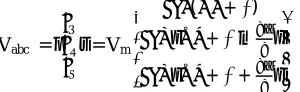
Vabc = = Vm
⎣ ⎢ ⎢
⎡ ( +ɸ)
+ɸ−
+ɸ+ ⎦⎥
⎥ ⎤
(25)
Where Vm = voltage magnitude ɸ= initial phase angle
Under this set of voltages, the fundamental of switching functions thus can be expressed as:
Sabc = = √
⎣ ⎢ ⎢
⎡ ( +ɸ)
+ɸ−
+ɸ+ ⎦⎥
⎥ ⎤
(26)
As it is seen from (25) and (26), the switching function fundamental components are in phase with input terminal voltage for this rectifier type. The input-output relationships of the DB rectifier are given as:
VDC = Vabc , (27)
Iabc = [ ]T = iDC (28)
Design of Three Phase Inverter
Figure 5 shows the circuit configuration of voltage source inverter. From this figure designing input and output variable using switching function concept. Inverter acts on two mode
of conduction :1. 1800 conduction mode, 2. 1200 conduction mode. Design is proposed in (Byoung-Kuk Lee and Mehrdad Ehsani, 2001). In this the conduction mode each switch conducts for 1800 of a cycle.
Fig.5. Three phase Inverter
Relationship between input and output variables is given as:
[ ]=TF.Vd. (29)
Vab , Vbc , Vca is Output Voltage
Iin = TF.[ ] (30)
where is input current and is o/p current. TF is transfer function of VSI .
Generally transfer function consists of several switching function is given as:
TF = [ … … … … .] (31)
In order to define the switching functions SPWM technique is applied as control strategy. Based on SPWM two switching function , is designing for inverter modeling. is used to express the , , and calculated the inverter line to line voltage ( , , ) and phase voltage ( , , ) . is designed for voltage across switch and load current ( , , ). In SPWM Block (carrier wave) is compared with (Sine wave) and generate , , (switching function of ).Using
, , switching function _ the voltage
, , is obtained. Equation is given as:
= . _ (32)
= . _ (33)
= . _ (34)
Inverter line to line voltage is given as (( , , ):
V = V - V , V = V - V , V = V - V (35)
Inverter phase voltage is given as ( , , ):
= ( + + ) (36)
[image:4.612.72.293.218.357.2] [image:4.612.61.211.414.460.2]V = V - V , V = V - V , V = V - V
Load current is given as ( , , ):
= , = , = (37)
Simulation Study
Simulation model is given in figure.6. It consists four model (wind model, Induction Generator, Three Phase Diode Rectifier, Three Phase Inverter). Wind model for generating wind speed, wind turbine for generating mechanical torque that drives Induction Generator. IG Model for converting mechanical energy into electrical energy, Three phase diode rectifier for converting AC to DC. Three phase Inverter Modeling for converting DC to AC Voltage. Converter and Inverter is used for synchronizing with power grid so that improve power quality and reduce harmonics (THD-total harmonic distortion) and increased efficiency is modled using Matlab /SIMULINK.
[image:5.612.323.543.70.224.2][image:5.612.69.297.288.392.2]
Fig.6. VSWT implemented in MATLAB/SIMULINK
[image:5.612.348.518.336.480.2]Fig .7. Step Speed, Ramp speed, Gust Speed and Noise Speed (m/sec)
Fig. 8.Wind Speed (m/sec) Performance Tests Under Varying Wind Speed
Table 3. Cp(ג, β) Characteristic Curve
Tip speed (ג) Cp(ג, β) for Pitch Angle (β = 0 Degree)
0.5 0.035
2.5 0.10
4.0 0.13
5.84 0.2413
6.96 0.3311
7.92 0.3925
8.6 0.4307
9.59 0.46
11.75 0.488 - CP-MAX
12.35 0.4855
13.56 0.4706
15.71 0.4211
17.61 0.2942
20 0.1011
21 -0.05
22 -0.1
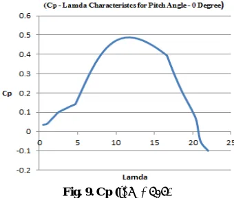
Wind Turbine rating is 2MW.From fig.8 Wind speed is varying from 3.5m/sec (cut in speed) to 11.35 m/sec .This speed is below base speed (12.35m/sec).Using simulation tool control wind speed for capturing maximum power from wind turbine. From Fig.9 Cp is 0.488 at
ג
= 11.75 it means efficiency of wind turbine is 48.8% (48.8 of wind energy is extracted from wind turbine) After increasing lamda (ג
) power goes down.Fig. 9. Cp (ג, β) Curve
From Fig.10 950 KW Mechanical power is generated that is (48.8% of Wind turbine rating), Mechanical Torque is below base torque.
[image:5.612.70.290.410.721.2] [image:5.612.326.537.535.701.2]From Fig.11 represent the three phase input voltage (220 V) is given to Induction Generator at 60 Hz. From design point of view convert 3- phase (abc) to 2- phase (dq0) using reference frame transformation theory and next transform dq generated voltage into three phase generated voltage.
Fig.11. Input Voltage (V), DQ axis Voltage (V), Output Voltage (V)
From Fig.12 represent three phase output current for load
resistance (3Ω) as we know that induction motor work as
generator for negative slip. In negative slip Rotor speed lies above synchronous speed and electromagnetic torque should be negative. From fig initially Tem is positive and ωr lies below base speed after that Tem is going negative and ωr is
increasing above base speed.
Fig.12. Output Current (Amp), Rotor Speed (pu), Electromagnetic Torque (Tem in pu)
Fig.13. Rectified Voltage (Vd in Volt), Rectified Current (Id in amp)
Fig.14. (a). Carrier wave, Sine Wave (A, B, C) (b).SF1-A, SF1-B, SF1-C
Fig.15. Inverter Phase Voltage (Van, Vbn, Vcn in Volt), Inverter Load Current ((Ia , Ib , Ic for RL Load).
From Fig.14 represent generation of pulse (SF1-A,SF1-B, SF1-C) using SPWM as we know that each switch in inverter is conducted at 120 degree. Based on this strategy Compare three sine wave (A,B,C) having phase difference 120 degree with carrier wave having frequency (1kHz) and generate three pulse (SF1-A,SF1-B, SF1-C) for controlling conduction of inverter. Based on equation generate inverter line to line and phase voltage.
Conclusion
In this paper we are analyzing VSWT performance in MATLAB/SIMULINK. Models of the subsystems of which a variable speed wind turbine consists were developed and practical values for the various parameters were given. It was concluded that both theoretical considerations and experimental evidence justify the representation of the two most important variable-speed wind turbine concepts with the same model in power system dynamics simulations. The integration of the developed model into a power system dynamics simulation software package was discussed and simulation results that were obtained with the derived model were analyzed When the response of the model to a measured wind.
REFERENCES
Seul-Ki Kim and Eung-Sang Kim, “PSCAD/EMTDC- Based Modelling and Analysis of a Gearless Variable Speed Wind Turbine,” IEEE Trans. On Energy Conversion, Vol. 22, No. 2, June 2007.
Slootweg, J. G., S. W. H. de Haan, H. Polinder and W. L. Kling, "General Model for Representing Variable Speed Wind,” Turbines in Power System Dynamics Simulations, "IEEE Trans. On Power Systems, VOL. 18, NO. 1, February 2003
Narayan Prasad Gupta, Preeti Gupta and Dr. Deepika Masand, “Power Quality Improvement Using Hybrid Active Power Filter for A DFIG Based Wind Energy Conversion System, ”Nirma University International Conference On Engineering, Dec 2012.
Yuya Izumi, Alok Pratap, Kosuke Uchida, Akie Uehara, Tomonobu Senjyuand, and Atsushi Yona, “A Control Method for Maximum Power Point Tracking of a PMSG-Based WECS using Online Parameter Identification of Wind Turbine, ”IEEE PEDS, Dec 2011.
Masaaki Sakui and Hiroshi Fujita, “An Analytical Method for Calculating Harmonic Currents of a Three- phase Diode-Bridge Rectifier with dc Filter, ”IEEE Trans. On Power Electronics, VOL. 9, NO. 6, November, 1994.
Byoung-Kuk Lee, Mehrdad Ehsani, “A Simplified Functional Simulation Model for Three-Phase Voltage-Source Inverter Using Switching Function Concept, ”IEEE Trans. On Industrial Electronics, VOL. 48, NO. 2, April 2001. Anderson, P. M., Anjan Bose. "STABILITY SIMULATION
OF WIND TURBINE SYSTEMS,"IEEE Transactions on Power Apparatus and Systems, Vol. PAS-102, No. 12, December 1983.
Chee – Mun Ong. “Dynamic Simulation of Electric Machinery Using MATLAB/SIMULINK “ West Lafayette, Indiana, Purdue University, pp. 167 – 243.