www.hydrol-earth-syst-sci.net/18/447/2014/ doi:10.5194/hess-18-447-2014
© Author(s) 2014. CC Attribution 3.0 License.
Hydrology and
Earth System
Sciences
Climate-driven interannual variability of water scarcity in food
production potential: a global analysis
M. Kummu1, D. Gerten2, J. Heinke2, M. Konzmann2, and O. Varis1
1Water & Development Research Group (WDRG), Aalto University, Espoo, Finland 2Potsdam Institute for Climate Impact Research (PIK), Potsdam, Germany
Correspondence to: M. Kummu ([email protected])
Received: 17 May 2013 – Published in Hydrol. Earth Syst. Sci. Discuss.: 3 June 2013 Revised: 30 December 2013 – Accepted: 3 January 2014 – Published: 5 February 2014
Abstract. Interannual climatic and hydrologic variability has
been substantial during the past decades in many regions. While climate variability and its impacts on precipitation and soil moisture have been studied intensively, less is known on subsequent implications for global food production. In this paper we quantify effects of hydroclimatic variability on global “green” and “blue” water availability and demand in global agriculture, and thus complement former studies that have focused merely on long-term averages. Moreover, we assess some options to overcome chronic or sporadic water scarcity. The analysis is based on historical climate forcing data sets over the period 1977–2006, while demography, diet composition and land use are fixed to reference conditions (year 2000). In doing so, we isolate the effect of interan-nual hydroclimatic variability from other factors that drive food production. We analyse the potential of food production units (FPUs) to produce a reference diet for their inhabitants (3000 kcal cap−1day−1, with 80 % vegetal food and 20 %
an-imal products). We applied the LPJmL vegetation and hy-drology model to calculate the variation in green-blue water availability and the water requirements to produce that very diet. An FPU was considered water scarce if its water avail-ability was not sufficient to produce the diet (i.e. assuming food self-sufficiency to estimate dependency on trade from elsewhere). We found that 24 % of the world’s population lives in chronically water-scarce FPUs (i.e. water is scarce every year), while an additional 19 % live under occasional water scarcity (water is scarce in some years). Among these 2.6 billion people altogether, 55 % would have to rely on in-ternational trade to reach the reference diet, while for 24 % domestic trade would be enough. For the remaining 21 % of
the population exposed to some degree of water scarcity, lo-cal food storage and/or intermittent trade would be enough to secure the reference diet over the occasional dry years.
1 Introduction
and hydrological droughts have been assessed globally, yet basically constrained to a purely hydroclimatological per-spective (Sheffield et al., 2009; Dai, 2011).
Sufficiency of blue water to meet certain demands can be measured with simple scarcity indices (Falkenmark et al., 1989; Falkenmark, 1997; Vörösmarty et al., 2000; Alcamo et al., 2003; Arnell, 2004; Oki and Kanae, 2006; Kummu et al., 2010). Although blue water and irrigation are cru-cial for global food production, still around 60 % of food is produced solely with green water resources on rainfed land (Rockström et al., 2009). Accordingly, green water con-tributes about 90 % to agricultural water consumption (Rost et al., 2008; Liu et al., 2009; Hoekstra and Mekonnen, 2012), such that a blue-water-based analysis only captures scarcities related to irrigation (and domestic and industrial uses). The importance of green water in food production has led to a quest for integrated green-blue water (GBW) scarcity indi-cators. Rockström et al. (2009) found a global GBW short-age by referring to a threshold of available GBW resources of 1300 m3cap−1yr−1, which is the amount of water needed to produce a “standard diet” (Falkenmark and Rockström, 2004). Gerten et al. (2011) developed a locally specific GBW scarcity indicator by taking explicitly into account the wa-ter productivity, i.e. the amount of GBW needed to produce a benchmark for hunger alleviation (3000 kcal cap−1day−1, assumed to consist of 80 % vegetal food and 20 % animal products).
All these studies have focused on water scarcity under long-term average climate conditions. Besides, recent global studies are available that have focused on average seasonal (i.e. intra-annual) blue water scarcity (Hanasaki et al., 2008; Wada et al., 2011b; Hoekstra et al., 2012), while interannual variability (i.e. the extent to which individual years diverge from the average condition) of blue water scarcity due to cli-matic variation has been analysed by Wada et al. (2011a). The latter study analysed the role of climate variability in the historical evolution (1960–2001) of blue water stress. It found that increased water demand was the main factor for increased water stress, while climatic variation was of-ten the main cause of extreme events, e.g. when prolonged dry period notably decreased the water availability. Wada et al. (2011a) fixed the population and water use for the year 1960, but still no assessment exists on how interannual hy-droclimatic variability affects more present water scarcity. We expect that this effect is notable; especially since the importance of interannual climate variability for food pro-duction and underlying water resources has been highlighted recently for many regions (e.g. Haile, 2005; Tubiello et al., 2007; Zhang et al., 2010).
We argue that it is imperative to improve the understand-ing of the variability and frequency of water scarcity in food production, as areas exposed to occasional scarcity re-quire essentially different response measures to overcome the food deficit than areas exposed to chronic water scarcity. Thus, quantitative knowledge of average water scarcity,
assessed for example over 30 yr (Gerten et al., 2011) or 10 yr (Rockström et al., 2009), might not reveal the areas that suf-fer water scarcity occasionally during dry years. On the other hand, these studies might classify areas to be water scarce although the stress is not present every year. Moreover, re-cently the climate variability, and related extreme climate events, have been reported to be increased in various parts of the globe (Coumou and Rahmstorf, 2012; IPCC, 2012) and their role in food production has been widely reported, e.g. in India (World Bank, 2012), Australia (Qureshi et al., 2013), and Eastern Africa (Moore et al., 2012).
In this paper we quantify the impact of interannual cli-matic variability on global GBW availability and require-ments for food production potential, using the GBW scarcity index introduced by Gerten et al. (2011). Our analysis is based on climate forcing data for the past 30 yr (1977–2006) while diet composition, population and land cover settings are fixed to specific reference conditions, in order to assess the isolated effect of climate variability on GBW scarcity. We thus aim to assess how the hydroclimatic variability impacts on food producing units’ (FPUs) potential to produce a given diet for their inhabitants. Moreover, we quantify whether the variability has changed over time by comparing two cli-matic periods (1947–1976 and 1977–2006), and use these results to assess whether water availability, requirements and scarcity would have been significantly different given the cli-matic variability of the former period. All calculations are performed with the LPJmL vegetation and hydrology model (Bondeau et al., 2007; Rost et al., 2008).
2 Data and methods
In this study we assess how present water demand for food production potential is influenced by hydroclimatic variabil-ity. To cover this variability (and its changes as observed in the past), we used climatic records for the past decades. As the purpose is to assess the isolated effect of climate vari-ability on green-blue water scarcity, we keep other variables (e.g. population, land use, diet and agronomic practices) con-stant at their year 2000 values. Introduced below are the methodologies and data used to conduct the study.
2.1 LPJmL model and data
of the reference (around year 2000) cropland distribution (Ramankutty et al., 2008) and maximum monthly irrigated and rainfed harvested areas (Portmann et al., 2010). Sea-sonal phenology of CFTs is simulated based on meteorologi-cal conditions. Agronomic practices are meteorologi-calibrated for the pe-riod around 2000 by adjusting three model parameters deter-mining the vegetation density and the maximum achievable leaf area index (LAI). This ensures that simulated yields best match those reported by FAOSTAT (see Fader et al., 2010 for details).
In LPJmL carbon fluxes and pools as well as water fluxes are modelled in direct coupling with vegetation dynamics. Possible effects of rising atmospheric CO2 concentration
on plant growth and water use efficiency could have been included, but the concentration was held constant here at 370 ppm, corresponding approximately to the year 2000 level to isolate the impact of climate (variability) on plant growth. Water requirements, water consumption (i.e. evapotranspira-tion, distinguished into transpiraevapotranspira-tion, evaporation and inter-ception loss) and crop water productivity (water consump-tion per unit of total biomass produced) are calculated for both irrigated and rainfed systems. On rainfed areas, all con-sumed water is green water per definition, whereas on areas equipped for irrigation, we distinguish the fractions of green and blue water. The latter is assumed to be withdrawn from rivers, reservoirs, lakes and shallow aquifers to the extent required by crops and unfulfilled by green water, consider-ing country-specific irrigation efficiencies. We assume that the irrigation water requirements of each CFT can always be met, with implicit contributions from fossil groundwater, river diversions or other large-scale water transports (details in Rost et al., 2008; Konzmann et al., 2013). It should be noted that this assumption may lead to overestimations in some parts of the world. River flow directions are determined as in Haddeland et al. (2011), and reservoir distribution and management as in Biemans et al. (2011).
The areal distribution of CFTs and grazing land, the cal-ibration parameters and the irrigation efficiencies are held constant at the year 2000 level throughout the simulation period. By doing so, we exclude any effects of agronomic practices and cropland expansion and thus allow for the separation of climate (variability) effects on GBW scarcity. Monthly values of temperature and fraction of cloud cover are taken from CRU TS 3.1 (Mitchell and Jones, 2005) and linearly interpolated to daily values. Monthly precipi-tation totals are taken from GPCC v5 (Rudolf et al., 2010; extended to cover the full CRU grid) and the number of monthly precipitation days is derived using the method from Heinke et al. (2013). Daily precipitation values are calculated from these two parameters by a statistical weather generator (Gerten et al., 2004), hence short-term droughts and their ef-fects on yields are not necessarily captured.
2.2 Analysis and reporting scales
The model results, with resolution of 0.5◦, are aggregated primarily to the FPU scale. FPUs divide the world into 281 sub-areas, being a hybrid between river basin and eco-nomic regions (Cai and Rosegrant, 2002; Rosegrant et al., 2002; De Fraiture, 2007) modified here as in Kummu et al. (2010). The final FPU set used includes 309 units with an average size of 467×103km2and an average population of 19.6 million people. Although the appropriate scale depends on market access and varies from region to region, we de-cided to focus on FPUs, as they are at a hydro-political scale within which the demand for water and food can be assumed to be managed (Kummu et al., 2010).
We introduce another three reporting scales to further anal-yse and present our results: countries, administrative regions, and hydrobelts. The administrative regions divide the world into 12 regions (see Fig. S1A in the Supplement) based on country borders. For this we use a regional data set origi-nating from the UN (2000), which was further modified by Kummu et al. (2010). The hydrobelts divide the world into eight zones determined by specific hydrological characteris-tics and formed based on river basin boundaries (Meybeck et al., 2013). The country and administrative region scales are used for a multi-scale analysis that reveals the spatial scale of need for food storage and/or trade as an option to reach the reference diet (see Sect. 2.5).
2.3 Calculation of green-blue water availability,
demand, and scarcity
occasions our approach might overestimate the blue water availability.
The total availability of GBW (i.e. green and blue water), aggregated to FPUs, is then compared with the amounts of GBW needed to produce the raw products for the reference diet of 3000 kcal cap−1day−1(with 80 % vegetal and 20 % animal-based share) for all inhabitants of the FPU, following the method developed by Gerten et al. (2011). The reference diet is based on the WHO and FAO recommended production level required to eradicate hunger (WHO, 2003; FAO, 2013c) and it includes the average food losses and waste (in terms of calories 24 %; Kummu et al., 2012). Subtracting this loss and waste from the total production gives a food consump-tion of around 2280 kcal cap−1day−1, being almost exactly the global average dietary energy requirement (country data averaged over 2007–2012) of 2245 kcal cap−1day−1defined
by FAO (2013c). We use the same reference diet, in terms of food supply, for all FPUs to follow the recommendations for hunger alleviation. It should be noted, however, that the actual calorie level and content of the diet vary from place to place. Moreover it is good to mention, that should the animal-based share be higher (lower) from the used 20 %, the pres-sure on water resources would also be higher (lower) due to the higher water consumption of animal-origin foodstuff (e.g. Hoekstra and Mekonnen, 2012).
Since we constrain our analysis to the effects of local hy-droclimatic variability on the production of a given diet, we omit the decoupling of food production potential and con-sumption areas. Although this does not reflect the current patterns, which are governed by international trade of agri-cultural commodities and associated virtual water trade, this analysis provides relevant information due to the following reasons: (i) security of domestic food supply for a possible emergency situation remains important for many countries; (ii) many low- and medium-income countries do not have sufficiently strong economies to enter global food markets and are thus mainly dependent on domestic food production, and (iii) globally more than 80 % of the food (energy-wise) is still consumed in the country it is produced in (based on Food balance sheets; FAO, 2013b). Thus, we argue, that know-ing the potential of reachknow-ing food self-sufficiency by FPUs and by countries is highly important information in assess-ing global and regional food security. Furthermore, by disre-garding current trade patterns in the analysis, we are able to identify the dependency of FPUs on this trade.
The GBW requirements result from the crop water produc-tivity (determined at grid cell level and influenced by climate and agronomic practices), the transpirational demand given by meteorological conditions, and the soil moisture. They are computed from both the water requirements to produce the vegetal calorie share on present cropland (represented by the CFTs) and from a provisional livestock sector. Contribu-tions from the latter come from both grazing land and crop-land (i.e. the shares used for feed production, assigned ac-cording to the scheme used in Gerten et al., 2011). The water
requirements from grazing land are computed slightly dif-ferently as compared to Gerten et al. (2011): here we weigh the green water available on each country’s and FPU’s graz-ing land accordgraz-ing to its water productivity, while Gerten et al. (2011) uses a water productivity relative to the global av-erage for grass.
GBW scarcity is given by the ratio between the GBW availability and the GBW requirements for producing the ref-erence diet. A region (FPU) is considered to be GBW scarce if its domestic GBW availability falls below the GBW re-quirements. It is acknowledged that in the case of GBW scarcity the gap between the availability and requirement would be small for some regions while large for others, when using average climate conditions. We argue that when tak-ing into account the interannual variability in climatic con-ditions, this sharp threshold is less problematic, as then the areas close to the threshold (on either side of it) are classified to be under occasional water scarcity (see more in Sect. 2.4).
2.4 Methods for analysing the variability and change in
variability
As GBW scarcity is assessed on the basis of GBW require-ments and GBW availability, it is important to understand the impact of climatic variability on both of them. To quan-tify this variability we use the coefficient of variation (CV; i.e. standard deviation divided by mean) that is comparable between different areas, and also between the three variables (GBW availability, requirements, scarcity). Further, we mea-sure the frequency of years when an FPU in question is under GBW scarcity (i.e. when it does not have enough water to produce the reference diet). This frequency analysis allows for the classification of the FPUs into three main groups, of which occasional GBW scarcity is further divided into four sub-groups:
1. no GBW water scarcity (enough GBW to produce the reference diet in all years);
2. occasional GBW water scarcity:
a. sporadic GBW scarcity (GBW scarcity in 1– 25 % of the years);
b. medium frequent GBW scarcity (GBW scarcity in 25–50 % of the years);
c. highly frequent GBW scarcity (GBW scarcity in 50–75 % of the years);
d. recurrent GBW scarcity (GBW scarcity in 75– 99 % of the years);
2000 - 2700 1300 - 2000 > 3400
2700 - 3400 650 - 1300< 650 > 34002700 - 3400 2000 - 27001300 - 2000 650 - 1300< 650
0 - 0.05
0.05 - 0.1 0.1 - 0.150.15 - 0.2 0.2 - 1.1 0 - 0.050.05 - 0.1 0.1 - 0.150.15 - 0.2 0.2 - 0.75
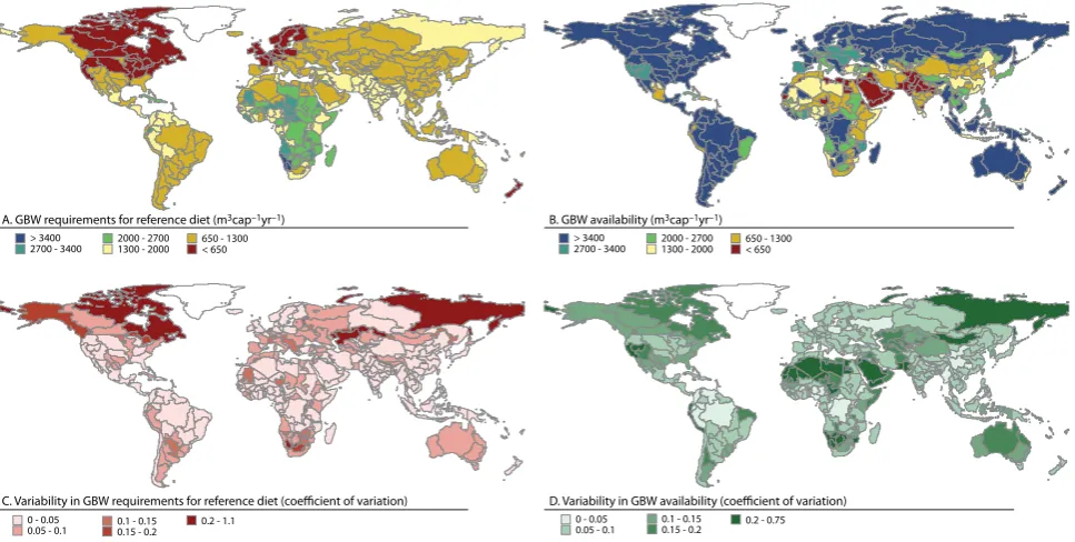
A. GBW requirements for reference diet (m3cap–1yr–1) B. GBW availability (m3cap–1yr–1)
[image:5.595.57.541.62.306.2]C. Variability in GBW requirements for reference diet (coefficient of variation) D. Variability in GBW availability (coefficient of variation)
Fig. 1. Green-blue water (GBW) requirements for reference diet and GBW availability. (A) Average GBW requirements over 30 yr climatic period; (B) average GBW availability over 30 yr climatic period; (C) variability in GBW requirements measured with coefficient of variation (CV); and (D) variability in GBW availability measured with CV.
the potential to produce enough food with available water resources under long-term average climate conditions. We also investigate whether there have been changes over time in GBW scarcity, as affected by changes in both the hydro-climatic variability and average hydrohydro-climatic conditions. In so doing, we first test with a one-way ANOVA whether the mean values of these two parameters are equal in two 30 yr climatic periods (1947–1976 and 1977–2006). Moreover, we analyse the changes in variability of GBW requirements and GBW availability within both 30 yr climatic periods. For that we use the Brown–Forsythe Levene’s test for equality of vari-ances (Brown and Forsythe, 1974), which assesses whether there is a difference in group variances between these two periods. All statistical tests are performed with SPSS v20. We also perform the frequency analysis of GBW scarcity for both climatic periods and compare those.
2.5 Response options and stress drivers: multi-scale
analysis and GBW matrix
We further conduct a multi-scale scenario analysis to scru-tinise possible response measures on how each FPU under GBW scarcity could theoretically reach the reference diet. The results from GBW scarcity analyses are used at FPU, country and regional scale to identify the possible response measures as follows (see also Table 2 in Sect. 3.3):
– Food self-sufficiency: an FPU that does not suffer from
any degree of GBW scarcity, hence without a need of measures to reach food self-sufficiency;
– Need for local food storage and/or intermittent trade:
if an FPU is subject to occasional scarcity but is self-sufficient under average climate conditions, it would need to store food in surplus years to overcome the deficit years and/or import (export) food in deficit (sur-plus) years;
– Need for domestic trade: if an FPU is not self-sufficient
under average climate conditions, but the country in which it is located is self-sufficient, it would need do-mestic trade to overcome the deficit years;
– Regional and inter-regional trade: if a country, in
which an FPU is located, is not self-sufficient under average climate conditions, an FPU is classified to need either regional trade (if the region of FPU in ques-tion is self-sufficient) or inter-regional trade (if it is not).
3 Results
3.1 Interannual variability of GBW scarcity
No scarcity Under scarcity
Never under scarcity 0 - 25% 25 - 50%
50 - 75% of years under scarcity 75-100%
Every year under scarcity
0° 23.4°N
23.4°S
0° 23.4°N
23.4°S
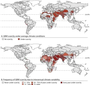
A. GBW scarcity under average climate conditions
[image:6.595.153.441.62.334.2]B. Frequency of GBW scarcity due to interannual climate variability
Fig. 2. Green-blue water (GBW) scarcity mapped by FPUs. (A) GBW scarcity under average climate conditions over 30 yr climatic period; and (B) frequency of GBW scarcity due to interannual climate variability. The marked latitudes represent the Tropic of Cancer (23.4◦N), Equator (0◦), and Tropic of Capricorn (23.4◦S). Note that the calculations were made for constant reference population and agronomical practices (year 2000 situation) but varying climate over the period of 1977–2006, in order to isolate the impact of climate variability on GBW scarcity.
the calibration, see Sect. 2.1). The requirements are low-est (<650 m3cap−1yr−1) in western Europe and large parts of North America, moderate (650–1300 m3cap−1yr−1) in southern parts of North America, South America and large part of Asia, and highest (>1300 m3cap−1yr−1) in north-ern parts of Latin America, Africa (except the northnorth-ernmost part) and South Asia (Fig. 1a). GBW availability per capita is lowest in very dry areas (e.g. North Africa, Middle East) and in highly populated places, such as in South Asia and China (Fig. 1b). High requirements often co-occur with low avail-ability (Fig. 1a and b), resulting in water-scarce conditions (Fig. 2).
The variability in GBW requirements is mostly rather low (CV<0.1) except for some areas (e.g. Canada, Siberia) where CV exceeds 0.2 (Fig. 1c). Variability of GBW avail-ability is much higher and spatially more heterogeneous, be-ing particularly high in dry areas, such as in North Africa, the Middle East, Australia, Central Asia and western China (Fig. 1d). The variability is, on the other hand, rather low or very low in large parts of South America, Europe, Sub-Saharan Africa, South Asia and eastern Asia (Fig. 1d).
We find that 34 % of the global population (year 2000 level) live in FPUs affected by GBW scarcity under long-term average climate conditions, i.e. the average GBW
requirements for the reference diet were larger than the av-erage available GBW resources (Table 1; Fig 2a). When analysing the frequency in GBW scarcity due to interannual climate variability, we find that 44 % of the world’s popu-lation live in FPUs under some degree of scarcity (Table 1; Fig. 2b). For about half of these people water is chronically scarce (equalling 24% of global population), while for the other half the scarcity is occasional (Table 1).
Table 1. Global population (in millions) under green-blue wa-ter (GBW) scarcity. Frequency of scarcity over the climatic pe-riod of 1977–2006 and over the 30 yr climatic pepe-riod before that (1947–1976). Bottom row (“average scarcity”) represents the GBW scarcity under average climate conditions within those climatic pe-riods. See also Figs. 2 and 4e. Note that the calculations were made for constant reference population and agronomical practices (year 2000 situation) but varying climate within the indicated time periods.
Population under GBW scarcity (in millions) Frequency 1977–2006 % of total 1947–1976 % of total
0 % 3471 57.4 % 3524 58.3 %
0–25 % 332 5.5 % 247 4.1 %
25–50 % 197 3.3 % 240 4.0 %
50–75 % 212 3.5 % 198 3.3 %
75–100 % 375 6.2 % 370 6.1 %
100 % 1456 24.1 % 1463 24.2 %
Total 6042 6042
Average scarcity 2027 33.6 % 1885 31.2 %
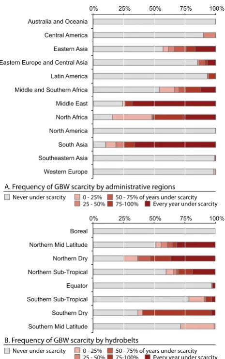
scarcity, while FPUs in Central America and Western Europe do not suffer long-term scarcity, but some are under occa-sional GBW scarcity (Figs. 2b and 3a).
When the results for frequency of GBW scarcity are aggre-gated by hydrobelts (see division in Fig. S1B in the Supple-ment), they reveal that in Northern and Southern Dry belts over half of the reference population suffer some degree of GBW scarcity, while in other belts less than half of the pop-ulation is exposed to water scarcity (Fig. 3b). In contrast, in the boreal and equatorial belts, 0 and 3 % of population, respectively, live under occasional scarcity. The belts in the Northern Hemisphere have relatively higher GBW scarcity than their southern analogues (Fig. 3b), mostly due to their much higher population densities (Kummu and Varis, 2011; Meybeck et al., 2013).
3.2 Change in GBW scarcity over time
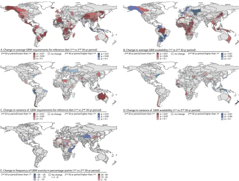
When comparing the 30 yr climatic period before 1977 to the climatic period of 1977–2006, we find that the average GBW requirements for the reference diet decreased statistically sig-nificantly (p <0.05) in 98 FPUs, while they increased in only 13 FPUs (Fig. 4a). It should be noted, however, that because the variability in GBW requirements is relatively small (Fig. 1c), these changes mostly result from rather small absolute changes (on average ∼5 % of the mean). The ar-eas with significant changes are concentrated in East Asia, Africa and along the west coast of Latin and North America. Changes in the variability of GBW requirements are less pro-nounced and significant only for a few FPUs (Fig. 4c). The most distinct changes in average GBW availability – namely decreases (p <0.05) – occurred in West Africa and South-east Asia (Fig. 4b). In large parts of Europe and in the south-ern part of South America, by contrast, the second period
Boreal
Northern Mid Latitude
Northern Dry
Northern Sub-Tropical
Equator
Southern Sub-Tropical
Southern Dry
Southern Mid Latitude
0% 25% 50% 75% 100%
0% 25% 50% 75% 100%
Australia and Oceania
Central America
Eastern Asia
Eastern Europe and Central Asia
South Asia Latin America
Middle and Southern Africa
Middle East
North Africa
North America
Southeastern Asia
Western Europe
A. Frequency of GBW scarcity by administrative regions
B. Frequency of GBW scarcity by hydrobelts Never under scarcity 0 - 25%
25 - 50%
50 - 75% of years under scarcity 75-100% Every year under scarcity
Never under scarcity 0 - 25% 25 - 50%
[image:7.595.49.288.173.294.2]50 - 75% of years under scarcity 75-100% Every year under scarcity
Fig. 3. Frequency of green-blue water (GBW) scarcity aggregated by (A) administrative regions, and (B) hydrobelts. See maps of the administrative regions and hydrobelts in Supplementary (Fig. S1A and S1B in the Supplement, respectively).
was wetter compared to the first one. The spatial pattern of changes, and the extent of those, in GBW variability (Fig. 4d) is less distinct than in the case of average GBW availability (Fig. 4b).
These changes in GBW requirements and GBW availabil-ity in response to changing climatic conditions are mirrored in the frequency of GBW scarcity (Fig. 4e). The frequency increases in large parts of Northern Africa and in Eastern China, while it decreases in Central Asia, in a few FPUs in Central America, and in large part of East Africa. Globally, the earlier climatic period resulted in a slightly lower popu-lation exposed to GBW scarcity (Table 1).
3.3 FPU dependency on trade and food storage
p < 0.01 p < 0.05 p < 0.1
p < 0.01 p < 0.05 p < 0.1 2nd 30-yr period lower than 1st 2nd 30-yr period higher than 1st
–38 - –20 –20 - –10 –2 - –10
20 - 48 10 - 20 2 - 10 2nd 30-yr period lower than 1st 2nd 30-yr period higher than 1st
p < 0.01 p < 0.05 p < 0.1
p < 0.01 p < 0.05 p < 0.1 2nd 30-yr period lower than 1st 2nd 30-yr period higher than 1st p < 0.01
p < 0.05 p < 0.1
p < 0.01 p < 0.05 p < 0.1
2nd 30-yr period lower than 1st 2nd 30-yr period higher than 1st p < 0.01 p < 0.05 p < 0.1
p < 0.01 p < 0.05 p < 0.1 2nd 30-yr period lower than 1st 2nd 30-yr period higher than 1st
E. Change in frequency of GBW scarcity in percentage-points (1st vs 2nd 30-yr period)
C. Change in variance of GBW requirements for reference diet (1st vs 2nd 30-yr period) D. Change in variance of GBW availability (1st vs 2nd 30-yr period) A. Change in average GBW requirements for reference diet (1st vs 2nd 30-yr period) B. Change in average GBW availability (1st vs 2nd 30-yr period)
no change
No change (–2 - 2)
no change
[image:8.595.56.537.60.423.2]no change no change
Fig. 4. Comparison of two 30 yr climatic periods (i.e. model forced by hydrometeorological data of 1947–1976 vs. 1977–2006). (A) Change in average green-blue water (GBW) requirements for the reference diet; (B) change in average GBW availability; (C) change in variance of GBW requirements; (D) change in variance of GBW availability; and (E) change in frequency of GBW scarcity. The change assessment in average values was conducted with One-way ANOVA and the change assessment in variability was conducted with the Brown–Forsythe Levene’s test. Note that the calculations were made for constant reference population and agronomical practices (year 2000 situation) but varying climate within the indicated time periods.
while for another 9 % the local storage and/or intermittent trade (import in deficit years and export in surplus years) would be enough (Table 2). The multi-scale analysis thus re-veals that FPUs inhabited by about two-thirds of the world’s population would have the potential to be independent of ei-ther domestic or international annual trade of food products if they chose to produce the reference diet for all their in-habitants on their own (and based on the products grown on their territory). Of those living in FPUs dependent on trade (34 % of global population), 70 % depend on international or interregional trade while for the rest, 30 % domestic trade (FPUs with 48 million people supported with national stor-age) would be enough to secure the reference food supply (Table 2). FPUs depending on interregional trade are located in South Asia and the Middle East, being the only regions not having the potential to produce intra-regionally the reference
diet for all inhabitants with available GBW resources on present cropland and grazing land (Fig. 5). The FPUs de-pendent on intra-regional trade are mainly located in North and East Africa and Central Asia, while the FPUs dependent only on domestic trade (i.e. trade within a nation) are mainly located in China. In Europe, Central America and Southeast Asia, the FPUs under occasional water scarcity would be able to reach food self-sufficiency with local storage and/or inter-mittent trade (Fig. 5).
4 Discussion and conclusions
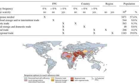
Table 2. Response options for FPUs, depending on the ability of to reach reference diet of 3000 kcal cap−1yr−1(see map in Fig. 5 and FPUs in GBW matrix in Fig. 6). Scarcity frequency refers to the frequency of GBW scarcity (see Fig. 2b) and average scarcity on GBW scarcity under average climate conditions (see Fig. 2a) over our study period of 1977–2006.
FPU Country Region Population
Scarcity frequency 0 % >0 % >0 % 0 % >0 % >0 %
Average scarcity no no yes no no yes no yes 106 %
No response needed X 3471 57.4 %
Local food storage and/or intermittent trade X 544 9.0 %
Domestic trade X X 563 9.3 %
National storage and domestic trade X X 48 0.8 %
Regional trade X X X 266 4.4 %
Inter-regional trade X X X 1163 19.0 %
Perennial food self-sufficiency
Response options to reach reference diet
Local storage and/or intermittent food trade
Domestic trade National storage + domestic trade
Regional trade Inter-regional trade
# of selected FPUs
100 510 891 232 20001 156
128
128 188
192
Fig. 5. FPU response options that would be needed to reach the local reference diet of 3000 kcal cap−1day−1(see Table 2 for more infor-mation). Selected FPUs are identified with their code; see Fig. 6 for their location in GBW matrix.
methodology, concept and knowledge on GBW scarcity and its impact on food production potential across the globe, as further discussed below. Our calculations indicate that 43 % of the planet’s population (relative to the year 2000 refer-ence population) dwell in areas characterised by at least some level of GBW scarcity, i.e. the GBW availability is insuffi-cient for producing the reference diet in the respective FPUs.
4.1 Uncertainties and evaluation of results
In this study we analysed the interannual variability in global water scarcity, as imposed by climatic variability, over sev-eral decades. We used the GBW scarcity indicator developed by Gerten et al. (2011), measuring the ability to produce a reference diet of 3000 kcal cap−1yr−1 within a given
spa-tial unit, e.g. an FPU, based on current agricultural areas, agronomic practices and population levels (fixed for a ref-erence period to separate the climate-only effect) with avail-able GBW resources. Prior to our study, the impact of inter-annual climate variability on global-scale water scarcity was assessed by Wada et al. (2011a), who used the year 1960 as a reference year to isolate the climatic impact from the an-thropogenic impact of the trend in blue water stress during
the period 1960–2001. In our study we used the year 2000 as a reference year and thus, we assessed the impact of interan-nual climate variability on considerably more recent condi-tions compared to Wada et al. (2011a). Furthermore, we con-sidered not only blue water but also green water for comput-ing water requirements and availabilities for food production, resulting in GBW scarcity estimations. Moreover, local crop water productivities were accounted for in calculating the GBW demand for the reference diet. Our analysis further ex-tends the current knowledge about water scarcity by assess-ing the interannual frequency of GBW scarcity (i.e. whether an area suffers from occasional or chronic water scarcity) in-stead of capturing only the average scarcity as resulting from longer-term average conditions, as was done in earlier studies (Vörösmarty et al., 2000; Alcamo et al., 2003; Arnell, 2004; Oki and Kanae, 2006; Falkenmark et al., 2009; Rockström et al., 2009; Kummu et al., 2010; Gerten et al., 2011).
accord with the few interannual variability analysis using sur-face observations of streamflow (Dettinger and Diaz, 2000) and precipitation (Fatichi et al., 2012). Fatichi et al. (2012) further used three gridded data sets (NCEP-NCAR, ERA-40, and GPCC Full Reanalysis) to assess the interannual vari-ability in precipitation; the patterns of the discharge variabil-ity found here agree rather well with those, except for east-ern Siberia where we suggest a higher variability in GBW availability (Fig. 1d) as compared to rather low precipitation variability. It should be noted, however, that although precip-itation is the key driver in GBW availability, other factors are relevant as well (e.g. Gerten et al., 2008), such as the mod-elled duration of crop growing periods.
We found that the GBW availability has changed over time due to changes in climate. The patterns of changes in the variability (Fig. 4d) of GBW availability were rather sim-ilar to the trend in the variability of precipitation as com-piled from seven databases for the years 1940–2009 (Sun et al., 2012). Further, the changes in mean GBW availabil-ity (Fig. 4b) were similar to observed trends in precipitation (IPCC, 2013) and modelled trends in blue water availability, i.e. river discharge (Gerten et al., 2008). It should be noted, however, that our timescale was somewhat different to these studies and we only mapped statistically significant changes. The GBW requirements for the reference diet were also found to change over time and are significantly lower in many areas during climatic period of 1977–2006 than in 1947–1976 (Fig. 4a), although the absolute change between these periods was not very large. Spatially explicit identifi-cation of the underlying mechanisms requires further anal-yses. However, the variability in GBW requirements did not change significantly between these two periods (Fig. 4c). The climate-driven changes in GBW availability and GBW re-quirements did not drastically alter the global number of peo-ple under GBW scarcity (Table 1), although local changes occurred (Fig. 4e).
Our analysis suggests that North America and Aus-tralia & Oceania were the only regions without GBW scarcity (Figs. 2b and 3a). This might be counter-intuitive at first glance, given the drought proneness of both areas, particu-larly Australia (Qureshi et al., 2013). This is probably due to two factors: (i) both areas are very large food exporters (FAO, 2013a) and it seems that even during the driest years the FPUs would have enough GBW resources to produce the reference diet for local population; and (ii) the FPU scale might, in some cases, be too large to identify local scarcity. Indeed, our method was not able to pick up very local, but still notable, GBW scarcity due to the used analysis scale, namely FPU. We do believe, however, that FPU is an ap-propriate scale to analyse demand for water and food. Thus for more local-scale analysis, a finer analysis scale should be used in future studies.
In summary, it should be noted that our findings are sub-ject to the model assumptions and parameterisations, espe-cially regarding the calculation of yields, which, however,
were calibrated here to minimise such biases. The forcing data used also exert strong influences on yield and water sources assessments (Biemans et al., 2009). Given these strictions, we recommend interpreting our results only at gional and global scales. To increase the robustness of our re-sults, multiple forcing data, and even multiple models, could be used. It should be further noted that we performed the calculations for a single year’s reference population, crop-land extent, and agronomic practices to reveal the impact of climate variability on GBW scarcity. Hence, we recommend that the diverse anthropogenic effects on GBW scarcity, and the historical trajectory of it, be investigated separately.
4.2 Response options beyond storage and trade
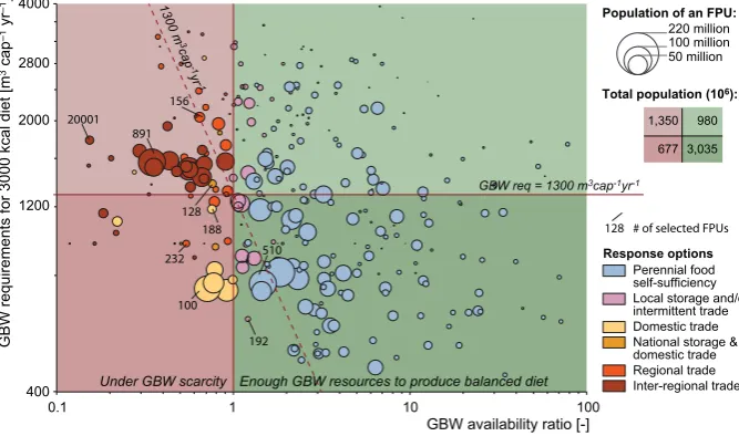
To facilitate the discussion of possible options to reach po-tential food self-sufficiency at FPU level, we designed the concept of a GBW matrix (see Fig. S2 in the Supplement), inspired by the blue water scarcity matrix developed by Falkenmark (1997). In the GBW matrix the GBW require-ments for the reference diet (y axis) are plotted against the GBW availability ratio (x axis; i.e. GBW availability vs. GBW requirements). The matrix thus also reveals the “distance” of each FPU to the scarcity threshold (Fig. 6). When plotting all FPUs grouped by response options (Ta-ble 2) in the GBW matrix, we see that the majority (90 %) of the FPUs that depend on international trade have GBW requirements larger than 1300 m3cap−1yr−1(Fig. 6). Thus, the possible response options for these FPUs, and for others with high GBW requirements, would involve improvements in agronomic practices. This would result in higher crop yield per used GBW resources. Another response option would be cropland expansion.
Indeed, Fader et al. (2013) found that many countries would possess the potential to produce the required food on their own – even under increasing population in the future – if agronomic practices would continuously improve at current rates. Yet, in some countries the local food self-sufficiency would require the expansion of their cropland. Cropland ex-pansion, however, introduces notable challenges to environ-mental sustainability (Wirsenius et al., 2010; Tilman et al., 2011) and the potential has been known to be quite lim-ited in most parts of the world already over several decades (Kendall and Pimentel, 1994; Pfister et al., 2011). Foley et al. (2011) conclude that when better agronomic practices (closing yield gaps and increasing cropping efficiency) are combined with shifting diets and reducing waste, global food security could be increased considerably. Political priorities related to food self-sufficiency should be brought into the picture as well, we argue; otherwise such discussions remain somewhat theoretical.
50 million 100 million 220 million
Population of an FPU: 1300 m
3
cap
-1
yr
-1
400 1200 2000 2800 4000
0.1 1 10
GBW requirements for 3000 kcal diet [m
3 cap
–1
yr
–1]
100 GBW req = 1300 m3cap-1yr-1
Total population (106):
677 1,350
3,035 980
GBW availability ratio [-]
Under GBW scarcity Enough GBW resources to produce balanced diet
Perennial food self-sufficiency
Response options
Local storage and/or intermittent trade
Domestic trade National storage & domestic trade Regional trade Inter-regional trade
# of selected FPUs
100 232
128 188
510
192 891
156 20001
[image:11.595.129.463.65.262.2]128
Fig. 6. FPUs mapped in the GBW matrix, grouped by response options. The location of an FPU is based on green-blue water (GBW) requirements for the reference diet (yaxis) and GBW availability ratio (xaxis; i.e. GBW availability vs GBW requirements) under average climate conditions. Thus, the FPUs with response option of “local storage and/or intermittent trade” are under occasional scarcity although not under average GBW scarcity. The dashed red line represents the threshold for GBW scarcity in Rockström et al. (2009), i.e. GBW availability of 1300 m3cap−1yr−1, and thus provides a comparison to their method. See Table 2 for more information of these options, and Fig. S2 in Supplement for the concept of the GBW matrix. The selected FPUs are identified with their code; see Fig. 5 for their location in a map. Note: log10 scale in both axes.
production of the reference diet (from a GBW resources view) would be either expanding the croplands (to get access to the green water on these areas) or transferring blue water from elsewhere. Long-distance water transfer is already hap-pening in many parts of the world, including China where water is being diverted from the rich south to the water-scarce north (Liu and Zheng, 2002). Northwest China and North China Plain are the areas where most of the country’s FPUs under GBW scarcity are located (Fig. 2b). Indeed, in these areas cropland expansion is no longer feasible (Liu et al., 2005; Pfister et al., 2011).
To verify some of our response option findings we re-flected our results to an assessment of countries’ food avail-ability and their trade dependency to meet the food energy consumption over the period of 1965–2005, conducted by Porkka et al. (2013). Their findings reveal, for example, that the food availability has increased notably in many of the ar-eas facing GBW scarcity in our analysis (e.g. North Africa and Middle East) since 1965. Many of the regions’ coun-tries have been able to raise their food availability from critically low (<2000 kcal cap−1day−1) to adequate level (>2500 kcal cap−1day−1) – mainly with the help of high food imports. At the same time, some other countries suffer-ing from GBW scarcity (e.g. in Eastern Africa, South Asia – i.e. countries with generally lower gross domestic pro-duction (GDP) than in the above-mentioned areas) have not managed to lift the food availability to an adequate level. Porkka et al. (2013, p. 7) indeed concluded that “average per cap GDP in countries that achieve sufficient food supply
by imports was approximately tenfold compared to countries with insufficient food supply and production”. Therefore, it is very much an economical issue whether a country can use the trade as a response option to overcome insufficient food production. When we compared our GBW scarcity results (Fig. 2b) with the food trade results of Porkka et al. (2013, p. 6), we found that all the countries in which the GBW-scarce FPUs are located were net food importers in year 2005.
4.3 Further research directions
dependency of many countries on agricultural trade to secure their food supply (Porkka et al., 2013). Moreover, the im-pact of producing non-food crops, such as fibres, should be accordingly analysed, since their role in many water-scarce FPUs is substantial.
We used FPUs as an analysis scale, as they are a hydro-political scale within which the demand for water and food can, in general, be assumed to be managed. In future studies the impact of resolution on the results should be studied. To find a single suitable resolution for a global scale might be difficult however, as the scale depends on food markets and infrastructure. While in some parts of the globe the markets are still very local, increasingly the food is coming from fur-ther away. This is particularly the case with large cities, and in their case the use of a very rough scale (e.g. 0.5◦) could result in misrepresented conclusions.
Many FPUs that are under GBW scarcity today, or are ap-proaching that, are facing rapid population growth and thus, the situation can be expected to become even more challeng-ing in the near future (Gerten et al., 2011; Fader et al., 2013; Suweis et al., 2013). It might actually already be so, since 14 yr have passed since the conditions of our population ref-erence year. The projected climate change, as well as popu-lation growth, thus add another stress dimension. This is par-ticularly the case in regions such as the Middle East, North-ern and SouthNorth-ern Africa, and parts of Australia. Therefore, it would be important to assess how the projected increase in hydroclimatic variability in the future (e.g. Boer, 2009; Wetherald, 2010) might impact on the frequency of GBW scarcity. As the future climate would concur with population projections, showing rapid growth in many areas under water scarcity (UN, 2011), much more FPUs would turn from wa-ter abundant to wawa-ter scarce (as suggested by Arnell, 2004; Arnell et al., 2011 for the river-basin scale).
Our analysis reveals the theoretical potential of FPUs to reach food self-sufficiency, or if that cannot be reached, the dependence level on either domestic or international food trade. We thus encourage the linking of our approach to in-vestigations on national and regional food policies across the globe in order to bridge the calculations of theoretical poten-tials to actual policy level priorities for meeting the demand for food.
Supplementary material related to this article is
available online at http://www.hydrol-earth-syst-sci.net/ 18/447/2014/hess-18-447-2014-supplement.pdf.
Acknowledgements. We thank our colleagues at Aalto University and PIK for their support and helpful comments. The comments and suggestions of the editor and reviewers are very much ac-knowledged. This work was funded by the Maa-ja vesitekniikan tuki ry, the postdoctoral funds and core funds of Aalto University, the Academy of Finland funded project SCART (grant no. 267463), Finnish Cultural Foundation under the Professor Pool scheme,
and the European Communities’ project CLIMAFRICA (grant no. 244240).
Edited by: T. J. Troy
References
Alcamo, J., Döll, P., Henrichs, T., Kaspar, F., Lehner, B., Rösch, T., and Siebert, S.: Global estimates of water withdrawals and avail-ability under current and future “business-as-usual” conditions, Hydrolog. Sci. J., 48, 339–348, 2003.
Arnell, N. W.: Climate change and global water resources: SRES emissions and socio-economic scenarios, Global Environ. Change, 14, 31–52, 2004.
Arnell, N. W., van Vuuren, D. P., and Isaac, M.: The implica-tions of climate policy for the impacts of climate change on global water resources, Global Environ. Change, 21, 592-603, doi:10.1016/j.gloenvcha.2011.01.015, 2011.
Barnett, T. P., Adam, J. C., and Lettenmaier, D. P.: Potential impacts of a warming climate on water availability in snow-dominated regions, Nature, 438, 303–309, 2005.
Biemans, H., Hutjes, R. W. A., Kabat, P., Strengers, B. J., Gerten, D., and Rost, S.: Effects of Precipitation Uncertainty on Dis-charge Calculations for Main River Basins, J Hydrometeorol., 10, 1011–1025, doi:10.1175/2008JHM1067.1, 2009.
Biemans, H., Haddeland, I., Kabat, P., Ludwig, F., Hutjes, R. W. A., Heinke, J., von Bloh, W., and Gerten, D.: Impact of reservoirs on river discharge and irrigation water supply during the 20th century, Water Resour. Res., 47, W03509, doi:10.1029/2009WR008929, 2011.
Boer, G. J.: Changes in Interannual Variability and Decadal Poten-tial Predictability under Global Warming, J. Climate, 22, 3098– 3109, doi:10.1175/2008JCLI2835.1, 2009.
Bondeau, A., Smith, P., Zaehle, S., Schaphoff, S., Lucht, W., Cramer, W., Gerten, D., Lotze-Campen, H., Müller, C., Reich-stein, M., and Smith, B.: Modelling the role of agriculture for the 20th century global terrestrial carbon balance, Global Change Biol., 13, 679–706, 2007.
Brown, C. and Lall, U.: Water and economic development: The role of variability and a framework for resilience, Nat. Resour. Forum, 30, 306–317, doi:10.1111/j.1477-8947.2006.00118.x, 2006. Brown, C., Meeks, R., Ghile, Y., and Hunu, K.: An Empirical
Analysis of the Effects of Climate Variables on National Level Economic Growth, The World Bank, Washington, D.C., 29 pp., doi:10.1596/1813-9450-5357, 2010.
Brown, M. B. and Forsythe, A. B.: Robust tests for equality of vari-ances, J. Am. Stat. Assoc., 69, 364–367, 1974.
Cai, X. and Rosegrant, M.: Global water demand and supply pro-jections, Part 1: A modeling approach, Water Int., 27, 159–169, 2002.
Carr, J. A., D’Odorico, P., Laio, F., and Ridolfi, L.: Recent History and Geography of Virtual Water Trade, PLoS ONE, 8, e55825, doi:10.1371/journal.pone.0055825, 2013.
Coumou, D. and Rahmstorf, S.: A decade of weather extremes, Nat. Clim. Change, 2, 491–496, 2012.
De Fraiture, C.: Integrated water and food analysis at the global and basin level. An application of WATERSIM, Water Resour. Manage., 21, 185–198, 2007.
Dettinger, M. D. and Diaz, H. F.: Global Characteristics of Stream Flow Seasonality and Variability, J. Hydrometeorol., 1, 289–310, doi:10.1175/1525-7541(2000)001<0289:GCOSFS>2.0.CO;2, 2000.
Fader, M., Rost, S., Müller, C., and Gerten, D.: Virtual water con-tent of temperate cereals and maize: Present and pocon-tential future patterns, J. Hydrol., 384, 218–231, 2010.
Fader, M., Gerten, D., Krause, M., Lucht, W., and Cramer, W.: Spatial decoupling of agricultural production and consumption: quantifying dependences of countries on food imports due to do-mestic land and water constraints, Environ. Res. Lett., 8, 014046, doi:10.1088/1748-9326/8/1/014046, 2013.
Falkenmark, M.: Meeting water requirements of an expanding world population, Philos. T. Roy. Soc. Lond. B, 352, 929–936, doi:10.1098/rstb.1997.0072, 1997.
Falkenmark, M. and Rockström, J.: Balancing Water for Humans and Nature: The New Approach in Ecohydrology, Earthscan, London, 2004.
Falkenmark, M., Lundqvist, J., and Widstrand, C.: Macro-scale wa-ter scarcity requires micro-scale approaches, Nat. Resour. Forum, 13, 258–267, 1989.
Falkenmark, M., Berntell, A., Jägerskog, A., Lundqvist, J., Matz, M., and Tropp, H.: On the Verge of a New Water Scarcity: A Call for Good Governance and Human Ingenuity, Stockholm In-ternational Water Institute – SIWI, Stockholm, 2007.
Falkenmark, M., Rockström, J., and Karlberg, L.: Present and future water requirements for feeding humanity, Food Security, 1, 59– 69, doi:10.1007/s12571-008-0003-x, 2009.
FAO: FAOSTAT – FAO database for food and agriculture, Food and agriculture Organisation of United Nations – FAO, Rome, 2013a. FAO: Food Balance Sheets, Part of FAOSTAT – FAO database for food and agriculture, Food and agriculture Organisation of United Nations – FAO, Rome, 2013b.
FAO: Food security indicators, available at http://www.fao.org/ economic/ess/ess-fs/ess-fadata/en/, last access: 19 April 2013, Food and Agriculture Organization of the United Nations – FAO, Rome 2013c.
Fatichi, S., Ivanov, V. Y., and Caporali, E.: Investigating Interan-nual Variability of Precipitation at the Global Scale: Is There a Connection with Seasonality?, J. Climate, 25, 5512–5523, doi:10.1175/JCLI-D-11-00356.1, 2012.
Foley, J. A., Ramankutty, N., Brauman, K. A., Cassidy, E. S., Ger-ber, J. S., Johnston, M., Mueller, N. D., O’Connell, C., Ray, D. K., West, P. C., Balzer, C., Bennett, E. M., Carpenter, S. R., Hill, J., Monfreda, C., Polasky, S., Rockstrom, J., Sheehan, J., Siebert, S., Tilman, D., and Zaks, D. P. M.: Solutions for a cultivated planet, Nature, 478, 337–342, doi:10.1038/nature10452, 2011. Gerten, D., Schaphoff, S., Haberlandt, U., Lucht, W., and Sitch, S.:
Terrestrial vegetation and water balance – hydrological evalua-tion of a dynamic global vegetaevalua-tion model, J. Hydrol., 286, 249– 270, doi:10.1016/j.jhydrol.2003.09.029, 2004.
Gerten, D., Rost, S., von Bloh, W., and Lucht, W.: Causes of change in 20th century global river discharge, Geophys. Res. Lett., 35, L20405, doi:10.1029/2008GL035258, 2008.
Gerten, D., Heinke, J., Hoff, H., Biemans, H., Fader, M., and Waha, K.: Global water availability and requirements for future food production, J. Hydrometeorol., 12, 885–899, doi:10.1175/2011JHM1328.1, 2011.
Gerten, D., Hoff, H., Rockström, J., Jägermeyr, J., Kummu, M., and Pastor, A. V.: Towards a revised planetary bound-ary for consumptive freshwater use: role of environmental flow requirements, Curr. Opin. Environ. Sustain., 5, 551–558, doi:10.1016/j.cosust.2013.11.001, 2013.
Haddeland, I., Clark, D. B., Franssen, W., Ludwig, F., Voß, F., Arnell, N. W., Bertrand, N., Best, M., Folwell, S., Gerten, D., Gomes, S., Gosling, S. N., Hagemann, S., Hanasaki, N., Harding, R., Heinke, J., Kabat, P., Koirala, S., Oki, T., Polcher, J., Stacke, T., Viterbo, P., Weedon, G. P., and Yeh, P.: Multimodel Estimate of the Global Terrestrial Water Balance: Setup and First Results, J. Hydrometeorol., 12, 869–884, doi:10.1175/2011JHM1324.1, 2011.
Haile, M.: Weather patterns, food security and humanitarian re-sponse in sub-Saharan Africa, Philos. T. Roy. Soc. B, 360, 2169– 2182, doi:10.1098/rstb.2005.1746, 2005.
Hanasaki, N., Kanae, S., Oki, T., Masuda, K., Motoya, K., Shi-rakawa, N., Shen, Y., and Tanaka, K.: An integrated model for the assessment of global water resources – Part 2: Applica-tions and assessments, Hydrol. Earth Syst. Sci., 12, 1027–1037, doi:10.5194/hess-12-1027-2008, 2008.
Heinke, J., Ostberg, S., Schaphoff, S., Frieler, K., Müller, C., Gerten, D., Meinshausen, M., and Lucht, W.: A new climate dataset for systematic assessments of climate change impacts as a function of global warming, Geosci. Model Dev., 6, 1689–1703, doi:10.5194/gmd-6-1689-2013, 2013.
Hirabayashi, Y., Kanae, S., Struthers, I., and Oki, T.: A 100-year (1901–2000) global retrospective estimation of the ter-restrial water cycle, J. Geophys. Res.-Atmos., 110, D19101, doi:10.1029/2004JD005492, 2005.
Hoekstra, A. Y. and Mekonnen, M. M.: The water foot-print of humanity, P. Natl. Acad. Sci., 109, 3232–3237, doi:10.1073/pnas.1109936109, 2012.
Hoekstra, A. Y., Mekonnen, M. M., Chapagain, A. K., Mathews, R. E., and Richter, B. D.: Global Monthly Water Scarcity: Blue Water Footprints versus Blue Water Availability, PLoS ONE, 7, e32688, doi:10.1371/journal.pone.0032688, 2012.
IPCC: Managing the Risks of Extreme Events and Disasters to Ad-vance Climate Change Adaptation, in: A Special Report of Work-ing Groups I and II of the Intergovernmental Panel on Climate Change, edited by: Field, C. B., Barros, V., Stocker, T. F., Qin, D., Dokken, D. J., Ebi, K. L., Mastrandrea, M. D., Mach, K. J., Plattner, G.-K., Allen, S. K., Tignor, M., and Midgley, P. M., Cambridge University Press, Cambridge, UK, and New York, NY, USA, 582 pp., 2012.
IPCC: Working Group I Contribution to the IPCC Fifth Assessment Report Climate Change 2013: The Physical Science Basis Sum-mary for Policymakers, Cambridge University Press, Cambridge,
UK and New York, NY, USA, vi+27, 2013.
Kendall, H. W. and Pimentel, D.: Constraints on the Expansion of the Global Food Supply, Ambio, 23, 198–205, 1994.
Kummu, M. and Varis, O.: The World by latitudes: a global analysis of human population, development level and environment across the north-south axis over the past half century, Appl. Geogr., 31, 495–507, doi:10.1016/j.apgeog.2010.10.009, 2011.
Kummu, M., Ward, P. J., de Moel, H., and Varis, O.: Is physical water scarcity a new phenomenon? Global assessment of wa-ter shortage over the last two millennia, Environ. Res. Lett., 5, 034006, doi:10.1088/1748-9326/5/3/034006, 2010.
Kummu, M., de Moel, H., Porkka, M., Siebert, S., Varis, O., and Ward, P. J.: Lost food, wasted resources: global food supply chain losses and their impacts on freshwater, crop-land, and fertiliser use, Sci. Total Environ., 438, 477–489, doi:10.1016/j.scitotenv.2012.08.092, 2012.
Liu, C. and Zheng, H.: South-to-north Water Transfer Schemes
for China, Int. J. Water Resour. Dev., 18, 453–471,
doi:10.1080/0790062022000006934, 2002.
Liu, J., Zehnder, A. J. B., and Yang, H.: Global consump-tive water use for crop production: The importance of green water and virtual water, Water Resour. Res., 45, W05428, doi:10.1029/2007WR006051, 2009.
Liu, X., Wang, J., Liu, M., and Meng, B.: Spatial heterogeneity of the driving forces of cropland change in China, Sci. China Ser. D, 48, 2231–2240, doi:10.1360/04yd0195, 2005.
Ma, Z. and Fu, C.: Global aridification in the second half of the 20th century and its relationship to large-scale climate back-ground, Sci. China Ser. D, 50, 776–788, doi:10.1007/s11430-007-0036-6, 2007.
Meybeck, M., Kummu, M., and Dürr, H. H.: Global hydrobelts and hydroregions: improved reporting scale for water-related issues?, Hydrol. Earth Syst. Sci., 17, 1093–1111, doi:10.5194/hess-17-1093-2013, 2013.
Mitchell, T. D. and Jones, P. D.: An improved method of con-structing a database of monthly climate observations and as-sociated high-resolution grids, Int. J. Climatol., 25, 693–712, doi:10.1002/joc.1181, 2005.
Moore, N., Alagarswamy, G., Pijanowski, B., Thornton, P., Lofgren, B., Olson, J., Andresen, J., Yanda, P., and Qi, J. G.: East African food security as influenced by future climate change and land use change at local to regional scales, Climatic Change, 110, 823– 844, doi:10.1007/s10584-011-0116-7, 2012.
Notaro, M.: Response of the mean global vegetation distribution to interannual climate variability, Clim. Dynam., 30, 845–854, doi:10.1007/s00382-007-0329-7, 2008.
Oki, T. and Kanae, S.: Global Hydrological Cycles and
World Water Resources, Science, 313, 1068–1072,
doi:10.1126/science.1128845, 2006.
Pfister, S., Bayer, P., Koehler, A., and Hellweg, S.: Projected water consumption in future global agriculture: Scenarios and related impacts, Sci. Total Environ., 409, 4206–4216, doi:10.1016/j.scitotenv.2011.07.019, 2011.
Piao, S., Friedlingstein, P., Ciais, P., de Noblet-Ducoudré, N., Labat, D., and Zaehle, S.: Changes in climate and land use have a larger direct impact than rising CO2 on global river runoff trends, P. Natl. Acad. Sci., 104, 15242–15247, doi:10.1073/pnas.0707213104, 2007.
Porkka, M., Kummu, M., Siebert, S., and Varis, O.: From food insufficiency towards trade-dependency: a historical anal-ysis of global food availability, PLoS ONE, 8, e82714, doi:10.1371/journal.pone.0082714, 2013.
Portmann, F. T., Siebert, S., and Döll, P.: MIRCA2000 – Global monthly irrigated and rainfed crop areas around the year 2000: A new high-resolution data set for agricultural and hy-drological modeling, Global Biogeochem. Cy., 24, GB1011, doi:10.1029/2008gb003435, 2010.
Qureshi, E. M., Hanjra, M. A., and Ward, J.: Impact of water scarcity in Australia on global food security in an era of climate change, Food Policy, 38, 136–145, doi:10.1016/j.foodpol.2012.11.003, 2013.
Ramankutty, N., Evan, A. T., Monfreda, C., and Foley, J. A.: Farm-ing the planet: 1. Geographic distribution of global agricultural lands in the year 2000, Global Biogeochem. Cy., 22, GB1003, doi:10.1029/2007GB002952, 2008.
Rockström, J., Falkenmark, M., Karlberg, L., Hoff, H., Rost, S., and Gerten, D.: Future water availability for global food production: The potential of green water for increasing re-silience to global change, Water Resour. Res., 45, W00A12, doi:10.1029/2007WR006767, 2009.
Rosegrant, M., Cai, X., and Cline, S.: World Water and Food to 2025, Dealing with Scarcity, International Food Policy Research Institute – IFPRI, Washington, D.C., USA, 2002.
Rost, S., Gerten, D., Bondeau, A., Lucht, W., Rohwer, J., and Schaphoff, S.: Agricultural green and blue water consumption and its influence on the global water system, Water Resour. Res., 44, W09405, doi:10.1029/2007WR006331, 2008.
Rudolf, B., Becker, A., Schneider, U., Meyer-Christoffer, A., and Ziese, M.: GPCC Status Report December 2010, Global Precip-itation Climatology Centre – GPCC, Offenbach, Germany, 7 pp., 2010.
Sakai, D., Itoh, H., and Yukimoto, S.: Changes in the Interannual Surface Air Temperature Variability in the Northern Hemisphere in Response to Global Warming, J. Meteorol. Soc. Jpn., 87, 721– 737, doi:10.2151/jmsj.87.721, 2009.
Sheffield, J., Andreadis, K. M., Wood, E. F., and Lettenmaier, D. P.: Global and Continental Drought in the Second Half of the Twentieth Century: Severity–Area–Duration Analysis and Tem-poral Variability of Large-Scale Events, J. Climate, 22, 1962– 1981, doi:10.1175/2008JCLI2722.1, 2009.
Sun, F., Roderick, M. L., and Farquhar, G. D.: Changes in the variability of global land precipitation, Geophys. Res. Lett., 39, L19402, doi:10.1029/2012GL053369, 2012.
Suweis, S., Rinaldo, A., Maritan, A., and D’Odorico, P.: Water-controlled wealth of nations, P. Natl. Acad. Sci., 110, 4230–4233, doi:10.1073/pnas.1222452110, 2013.
Tilman, D., Balzer, C., Hill, J., and Befort, B. L.: Global food de-mand and the sustainable intensification of agriculture, P. Natl. Acad. Sci., 108, 20260–20264, doi:10.1073/pnas.1116437108, 2011.
Tubiello, F. N., Soussana, J. F., and Howden, S. M.: Crop and pas-ture response to climate change, P. Natl. Acad. Sci. USA, 104, 19686–19690, doi:10.1073/pnas.0701728104, 2007.
UN: United Nations World Macro Regions and Components, United Nations – UN, http://unstats.un.org/unsd/methods/m49/ m49regin.htm (last access: May 2013), 2000.
UN: World Population Prospects: The 2010 Revision, Population Division of the Department of Economic and Social Affairs of the United Nations – UN – Secretariat, available at http://esa.un. org/unpp (last access: March 2012), 2011.
Vörösmarty, C. J., Green, P., Salisbury, J., and Lammers, R. B.: Global Water Resources: Vulnerability from Climate Change and Population Growth, Science, 289, 284–288, 2000.
Wada, Y., van Beek, L. P. H., and Bierkens, M. F. P.: Modelling global water stress of the recent past: on the relative impor-tance of trends in water demand and climate variability, Hy-drol. Earth Syst. Sci., 15, 3785–3808, doi:10.5194/hess-15-3785-2011, 2011a.
Wada, Y., van Beek, L. P. H., Viviroli, D., Dürr, H. H., Weingartner, R., and Bierkens, M. F. P.: Global monthly water stress: 2. Water demand and severity of water stress, Water Resoures Research 47, W07518, doi:10.1029/2010WR009792, 2011b.
Ward, P. J., Beets, W., Bouwer, L. M., Aerts, J. C. J. H., and Renssen, H.: Sensitivity of river discharge to ENSO, Geophys. Res. Lett., 37, L12402, doi:10.1029/2010GL043215, 2010. Ward, P. J., Eisner, S., Flörke, M., Dettinger, M. D., and Kummu,
M.: Annual flood sensitivities to El Niño-Southern Oscilla-tion at the global scale, Hydrol. Earth Syst. Sci., 18, 47–66, doi:10.5194/hess-18-47-2014, 2014.
Wetherald, R.: Changes of time mean state and variability of hydrol-ogy in response to a doubling and quadrupling of CO2, Climatic Change, 102, 651–670, doi:10.1007/s10584-009-9701-4, 2010. WHO: Diet, nutrition and the prevention of chronic diseases, World
Health Organisation – WHO, Geneva, Switzerland, 149 pp., 2003.
Wirsenius, S., Azar, C., and Berndes, G.: How much land is needed for global food production under scenarios of dietary changes and livestock productivity increases in 2030?, Agr. Syst., 103, 621–638, doi:10.1016/j.agsy.2010.07.005, 2010.
World Bank: Turn Down the Heat: Why a 4◦C Warmer World Must
be Avoided, A Report for the World Bank by the Potsdam Insti-tute for Climate Impact Research and Climate Analytics, Wash-ington, D.C., 106 pp., 2012.
Zachos, J., Pagani, M., Sloan, L., Thomas, E., and Billups, K.: Trends, Rhythms, and Aberrations in Global Climate 65 Ma to Present, Science, 292, 686–693, doi:10.1126/science.1059412, 2001.