TSP Solver using Constructive Method of Heuristic Approach

TSP Solver using Constructive Method

of Heuristic Approach

Chetan Chauhan

India

Ravindra Gupta

India

Kshitij Pathak

India

ABSTRACT

The Traveling salesperson problem (TSP) is one of the problem in mathematics and computer science which had drown attention as it is easy to understand and difficult to solve. In this paper, we implemented a heuristic approach for TSP using constructive method which generates satisfactory results in asymptotically linear time. Earlier work consider complete graph as a input to TSP. TSP solver generated by proposed approach can work with non-complete graph as well as complete graph.

Keywords

Traveling Salesman problem, Heuristic approach, Constructive method, Exact Solution Approaches

1.

INTRODUCTION

Traveling Salesman Problem (TSP) is classical and very famous problem. It is most widely studied problem in Combinatorial Optimization [1]. It has been studied intensively in both Computer Science and Operations Research since 1950s as a result of which a large number of techniques were developed to solve this problem. The idea of problem is to find shortest route of salesman starting from a given city called origin city, visiting n cities only once and finally arriving at origin city.

TSP is represented by complete as well as non-complete edge-weighted graph G=(V,E) with V being set of n=|V| nodes or vertices representing cities and EV×V being set of directed edges or arcs. Each arc (i, j)E is assigned value of length dij which is distance between cities i and j with i, jV . The goal in TSP is thus to find minimum length Hamiltonian Circuit [2]of graph, where Hamiltonian Circuit is a closed path visiting each of n nodes of G exactly once. Thus, an optimal solution to TSP is permutation π of node indices {1,...,n} such that length f(π) is minimal, where f(π)is given by,

( ) ∑

2.

RELATED WORK

In 1757, the first appearances of TSP in the mathematical literature have been seen in the paper by the great Leonard Euler and this paper concerns a solution of the knight’s tour problem in chess [4].In 1800’sIrish mathematician sir W. R. Hamilton and the English mathematician T. P. Kirkman treated mathematical problems related to the TSP. In 1832 B.F. Voigt goes through 47 German cities in The German handbook[5].

In 1930,The general form of the TSP has been appeared in Vienna and at Harvard, notably by Karl Menger, who defines the problem, considers the obvious brute-force algorithm, and observes the non-optimality of the nearest neighbor heuristic. Shortly after this the TSP became popular among mathematicians at Princeton University. In 1934, According to Merrill Flood and A. W. Tucker, Hasseler Whitney

presented a seminar on the name of this problem at Princeton University [6].

Merrill Flood tried to obtain near optimal solutions in reference to routing of school buses in 1937 at Columbia University. In the 1950s and 1960s, the problem became increasingly popular in scientific and in mathematician circles in Europe and the USA. California experts, George Dantzig, Delbert Ray Fulkerson and Selmer M. Johnson, were part of an exceptionally strong and influential center for the new field of mathematical programming, housed at the RAND Corporation in Santa Monica. They expressed TSP as an integer linear program and developed the cutting plane method for its solution. Using these new methods they took up the computational challenge of TSP, solving a 49-city instance by hand to optimality by constructing a tour and proving that no other tour could be shorter [7].

In 1962, A contest organized by Procter & Gamble consisting of a problem instance of 33 cities in USA having price $ 10,000 for the shortest solution. In 1970, Held and Karp developed a one-tree (A tree containing exactly one cycle) relaxation which provides a lower bound within 1 % from the optimal. In 1972, Karp proved the NP-completeness of the Hamiltonian Cycle Problem (HCP) from which the NP-completeness of the TSP follows almost directly [8].

In 1973, Lin and Kernighan proposed a variable-depth edge exchanging heuristic for refining an initial tour. In 1976, Christofides published a tour construction method that achieves a 3/2-approximation. Apart from the euclidean TSP this is still the tightest approximation ratio known [9]. In article [10] introduces the random, local search technique known as “Simulated Annealing”. In article [11], one of the first publications discussing “Neural Network” algorithms.

In 1990, a new highly efficient variant of the k-d tree data structure developed by Bentley, which is used for proximity checking and he was working on for the TSP on heuristics approach[12].In 1991, Reinelt composed and published TSPLIB [13], a library consisting many of the test problems that studied over the many last years [14].

In 1992, David Applegate, Robert Bixby, Vašek Chvátal and William Cook solved a 3038 TSP city instance by using the exact TSP solver program with optimality.In1996,Arora derived the first Polynomial Time Approximation Scheme (PTAS) for the euclidean TSP. In 1998 Keld Helsgaun developed highly improved and efficient extension of the Lin-Kernighan heuristic algorithm, called Lin-Kernighan- Helsgaun (LKH).

contributed by Applegate, Bixby, Chvátal, Cookand Helsgaun. In 2005, Cook and others computed an optimal tour through a 33,810-city instance given by a microchip layout problem. In 2006, 85,900-city instances solved and proven optimal using LKH and Concorde [21].The current record an 85,900-city tour that arose in a chip-design application [22].

3.

TSP SOLVER

There are basically two types of TSP solver.

3.1Exact Solvers

The main characteristics of Exact Solver is a guarantee of finding the optimal solution at the expense of running time and space requirement. Example of exact solver is branch and bound, the cutting plane, branch and cut, dynamic programming, brute force method etc.

3.2

Non-exact Solvers

The main characteristic of these solvers is that it offers potentially non-optimal but gives the typically faster solutions. In other words it is opposite trade-off of the exact solvers. Non-exact solvers can be subdivided into two type:

Approximation Algorithms These algorithms come with a

worst case approximation factor for the found solution. These algorithm does not gives the correct result but gives fast result. The two traditional methods for solving the TSP are a pure MST based algorithm and Minimum Matching Problem (MMP). Both methods are restricted to the MTSP as they depend on the triangle inequality. The PTAS for Euclidean TSP is mainly a theoretical result due to its prohibitive running time.

Heuristic Algorithms ‘heuristic’ is a Greek word which

meant “Serving to discover or stimulate investigation” its original form was heuriskein which meant “to discover”. In heuristics, one endeavours to understand the process of solving problems, especially the mental operation of a human problem-solver, which is most useful in this process [15].

There are several reasons for using heuristic method for solving problem. They are as follows [16]:

1. The mathematical problem is such that analytic (closed form) or iterative solution procedure is unknown. 2. Although an exact analytic or iterative solution

procedure may exist, it may be computationally prohibitive to use or it may be unrealistic in its data requirements. This is particularly true of enumerative methods, which in theory, are often applicable where analytic and iterative procedures cannot be found. 3. The heuristic method is simpler for the decision maker to

understand, hence, it markedly increases the chance of implementation.

4. For a well defined problem that can be solved optimally, a heuristics method can be used for learning purposes. 5. In implicit enumeration approaches, a good starting

solution can give a bound that drastically reduces the computational effort; heuristics can be used to give such “good” starting point.

6. Heuristics may be used as part of an iterative procedure that guarantees the finding of an optimal solution. Two distinct possibilities exist:

 To easily obtain an initial feasible solution.

 To make a decision at an intermediate step of an exact solution procedure. There are a large number of “proven” approaches in Heuristics, which are discussed below [16, 17, 18, 19]

1. Decomposition methods

2. Inductive methods

3. Feature extraction (or reduction) methods 4. Methods involving model manipulation 5. Constructive methods

6. Local improvement methods

Advantages and limitations of heuristics methods Some advantages of using heuristics are as follows [20]:

 These methods are simple to understand and easier to implement so these help to save the formulation time as well as save computer running time(speed).  Heuristics help in training people to be creative and

come up with heuristics for other problems.  These methods save the programming and storage

requirement on the computers as well as produce multiple solutions in less time.

However, there are some limitation in using heuristic in that:  Heuristics methods consider all possible

combination that’s why difficult to be achieved in practical problem.

 These methods take sequential decision choices that can fail to each choice of future consequences.  Heuristics lacks a global perspective because “local

improvement” can short-circuit the best solution.  Interdependencies of parts of a system are ignored

by the heuristics. This can sometimes have a profound influence on solution to the problem in the total system.

4.

PROPOSED SOLUTION

This paper implements the constructive method for finding a satisfactory solution to the traveling salesman problem. The basic idea of a constructive method is to literally build up to a single feasible solution, often in a deterministic, sequential fashion. This solution can be applied to non complete connected graph as well as complete connected graph.

The constructivemethod proceeds as follows.

Traveling salesman problem using constructive method //Assume S as initial city, n=total number of cities, C=1

for each vertex V ε (G)-{S}

do

color[V]=white //make all node to white color

end for

color[S]=gray //make source node to gray color Total_dist=0 //initialize the total distance Π[C]=S // Π contains the path of TSP C++

Q ←{S} //starting node put in queue

while(Q≠0) do

u← dequeue (Q) //delete in queue tempd=∞

for all node n adjacent to u //check all neighbor

do

ifcolor[n] =white then

if (temp>dist[u,n]) then

{tempd= dist[u,n] π[C]=n }

End For

color [π[C]]=gray //change the color of nearest neighbor Total_dist=Total_dist + dist[π[C-1],π[C]]

Enqueue(π[C]) //put in queue C++

End While

Example 1

City or Town Point A

Point B

Point C

Point D

Point A 0 2 5 4

Point B 1 0 9 6

Point C 3 21 0 25

Point D 1 1 2 0

Applying the Constructive method step by step:-

Here V={A,B,C,D}, C=1 Source, S=A Total_dist=0 Colors of node

Index 1 2 3 4

Nodes A B C D

Color Gray White White White Π contains the path of TSP

Index1234 A For C=2 Queue=A

Check until queue is empty u←A

tempd=∞

check all the adjacent node having white color for A calculate cost and those cost is minimum then change the color of those node to gray, here we have node B

Colors of node

Index 1 2 3 4

Nodes A B C D

Color Gray Gray White White Total_dist=0+2=2

Π contains the path of TSP Index 1 2 3 4

A B Similarly, we get

Index 1 2 3 4

Nodes A B C D

Color Gray Gray Gray Gray Total_dist=13

Π contains the path of TSP Index 1 2 3 4

A B D C

The shortest path starting from city A is as follows:- A→B→D→C→A

4.1

Implementation

The algorithm is implemented in oracle fusion middleware.

Fig 1 Cost matrix

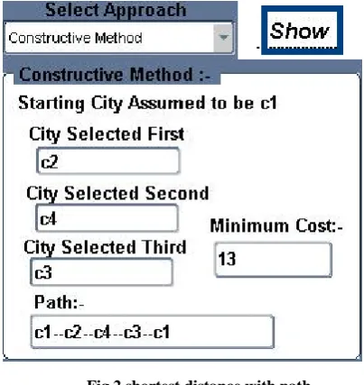
Figure 1 shows the cost matrix of TSP for 4 cities. In this figure first column and second column represent the city denoted by C1, C2, C3 and C4. In third column we have distance between two cities, for example, first row represent the distance between city C1 and C2 is 2.

Figure 2 represents the result of constructive method. This shows the shortest distance and suggested path for traveling salesman.

Fig 2 shortest distance with path

5.

COMPARISON WITH DYNAMIC

PROGRAMMING

5.1

Correctness

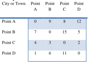
Dynamic programming always gives the correct solution while constructive method does not provide the correct solution always but gives the quick solution. For example

Example 2

City or Town Point A

Point B

Point C

Point D

Point A 0 9 8 12

Point B 7 0 15 5

Point C 4 3 0 2

Point D 1 6 11 0

By applying the dynamic programming method we get:-

Let IS=A g(B, ∅)= CBA=7 g(C, ∅)= CCA=4 g(D, ∅)= CDA=1

g(B, {C, D})=min(CBC + g(C, D),CBD + g(D, C)) { since g(C, D)= CCD + g(D,∅)=2+1=3 g(D, C)=CDC + g(C,∅)=11+4=15 } g(B, {C, D})=min(15+3,5+15)

=min(18, 20) =18

Similarly, we get g(C, {B, D})=9 g(D, {B, C})=21

g(A, {B, C, D})=min(CAB + gBCD, CAC+ gCBD , CAD + gDCB) =min(9+18,8+9,12+21)

=min(27, 17, 33) =17

The shortest path starting from city A is as follows:-

A→C→B→D→A(as shown in implementation in Fig 3)

Applying the Constructive method step by step:- Here V={A,B,C,D}, C=1

Source, S=A Total_dist=0 Colors of node

Index 1 2 3 4

Nodes A B C D

Color Gray White White White

Π contains the path of TSP Index 1 2 3 4

A For C=2 Queue=A

Check until queue is empty u←A

tempd=∞

check all the adjacent node having white color for A calculate cost and those cost is minimum then change the color of those node to gray, here we have node B

Colors of node

Index 1 2 3 4

Nodes A B C D

Color Gray White Gray White Total_dist=0+8=8

Π contains the path of TSP Index 1 2 3 4

A C Similarly, we get

Index 1 2 3 4

Nodes A C D B

Color Gray Gray Gray Gray Total_dist=23

Π contains the path of TSP Index 1 2 3 4

A C D B

The shortest path starting from city A is as follows:-

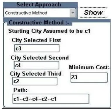
A→C→D→B→A(as shown in implementation in Fig 4)

Fig 4 shortest distance with path using Constructive method

5.2

Complexity

Complexity of dynamic programming approach is Ο(n2

2n) while the complexity of constructive method is Ο(V+E) where V is set of cities and E is edge between the cities. Fig 5 represents a graph that shows the comparison between execution time when using dynamic programming approach and constructive method approach by increasing number of nodes. As it is clear from the figure 5 that constructive method give quick solution, but not the optimal one in every case.

Fig 5 Comparison between Constructive Method and Dynamic Programming Approach

6.

FUTURE WORK

The advantage of dynamic programming approach is that it gives the correct and optimal solution and the advantage of constructive method is that it always gives the quick solution. In future we plan a solution of TSP using dynamic programming approach and try to use constructive method in intermediate step to achieve the correct with optimal solution with reasonable time.

7.

CONCLUSION

This paper uses constructive method for finding solution to travelling salesman problem. The major advantage of this is to get a fast feasible solution and even this approach can be applied to non-complete graph. The complexity of the

algorithm is

θ

between the cities.

REFERENCES

[1] Applegate, D. L., Bixby, R. E., Chvảtal, V. & Cook, W. J. (2006). The Traveling Salesman Problem: A Computational Study, Princeton University Press, Princeton, New Jersey.

[2] CormenT. H., Leiserson, C. E., Rivest, R. L. & Stein, C. (2001). Introduction to Algorithms, Second Edition, MIT Press Cambridge, Massachusetts.

[3] The Traveling Salesman Problem: A case study in local optimization by David S. Johnson and Lyle A. McGeoch 1995

[4] D.L. Applegate, R.E. Bixby, V.Chv´atal, W.J. Cook, The Traveling Salesman Problem, A Computational Study, Princeton University Press, Princeton and Oxford, 2006.

[5] Applegate, D. L., R. E. Bixby, V. Chvátal, and W. J. Cook (2007). The Traveling Salesman Problem: A Computational Study (Princeton Series in Applied Mathematics)., Chapter 1–5,12–17. Princeton, NJ, USA: Princeton University Press.

[6] Dantzig, G., R. Fulkerson, and S. Johnson (1954). Solution of a large scale traveling salesman problem. Technical Report P-510, RAND Corporation, Santa Monica, California, USA.

[7] Cook, William. "History of the TSP." The Traveling Salesman Problem. Oct 2009. Georgia Tech, 22 Jan 2010. <http://www.tsp.gatech.edu/index.html>.

[8] Karp, R. M. (1972). Reducibility among combinatorial problems. In R. Miller and J. Thatcher (Eds.), Complexity of Computer Computations, New York, USA., pp. 85–103. Plenum Press.

[9] Christofides, N. (1976). Worst-case analysis of a new heuristic for the traveling salesman problem. Technical Report Report 388, Graduate School of Industrial Administration, Carnegie-Mellon University, Pittsburg.

[10]S. Kirkpatrick, C. D. G. J. and M. P. Vecchi (1983, May). Optimization by simulated annealing. Science 220(4598), 671–680.

[11]Hopfield, J. J. and D. W. Tank (1985). “Neural” computation of decisions in optimization problems. Biological Cybernetics 52, 141–152. 10.1007/BF00339943.

[12]Bentley, J. L. (1992). Fast algorithms for geometric traveling salesman problems. ORSA Journal on Computing 4(4), 387–411.

[13] http://www.iwr.uniheidelberg.de/groups/comopt/softwar-e/TSPLIB95/

0 2000 4000 6000 8000 10000 12000 14000 16000

4 5 6 7 8 9 10

E

xec

u

tion

t

im

e

in

m

s

No. of Nodes

Dynamic Programming

[14]Reinelt, G. (1991, Fall). Tsplib - a traveling salesman problem library. ORSA, Journal On Computing 3(4), 376–384.

[15]K. N. Krishnaswamy, AppaIyer Sivakumar, M. Mathirajan (2009). Management Research Methodology: Integration of Methods and Techniques. Pearson Education India

[16]Edward A. Silver, R. Victor, V. Vidal, Dominique de Werra (1980). A tutorial on heuristic methods. European Journal of Operational Research Volume 5, Issue 3, Pages 153–162

[17]Michael Ball, Michael Magazine (1981). The design and analysis of heuristics. Networks Volume 11, Issue 2, pages 215–219.

[18]Weiner, P., "Heuristics", Networks 5 (1975) 101-103. [621/H].

[19]Stelios H. ZANAKIS, James R. EVANS, Alkis A. VAZACOPOULOS (1989). Heuristic methods and applications: A categorized survey. European Journal of Operational Research 43 , 88-110 North-Holland

[20]Turban, E. (1990). Decision support and expert system. Macmillan series in information system.

[21]Chetan Chauhan, Ravindra Gupta and Kshitij Pathak. Article: Survey of Methods of Solving TSP along with its Implementation using Dynamic Programming Approach. International Journal of Computer Applications 52(4):12-19, August 2012. Published by Foundation of Computer Science, New York, USA.