c
2002 Hindawi Publishing Corporation
Dynamic Bayesian Networks for Audio-Visual
Speech Recognition
Ara V. Nefian
Intel Corporation, Microprocessor Research Labs, 2200 Mission College Blvd., Santa Clara, CA 95052-8119, USA Email: [email protected]
Luhong Liang
Intel Corporation, Microcomputer Research Labs, Guanghua Road, 100020 Chaoyang District, Beijing, China Email: [email protected]
Xiaobo Pi
Intel Corporation, Microcomputer Research Labs, Guanghua Road, 100020 Chaoyang District, Beijing, China Email: [email protected]
Xiaoxing Liu
Intel Corporation, Microcomputer Research Labs, Guanghua Road, 100020 Chaoyang District, Beijing, China Email: [email protected]
Kevin Murphy
Computer Science Division, University of California, Berkeley, Berkeley, CA 94720-1776, USA Email: [email protected]
Received 30 November 2001 and in revised form 6 August 2002
The use of visual features in audio-visual speech recognition (AVSR) is justified by both the speech generation mechanism, which is essentially bimodal in audio and visual representation, and by the need for features that are invariant to acoustic noise pertur-bation. As a result, current AVSR systems demonstrate significant accuracy improvements in environments affected by acoustic noise. In this paper, we describe the use of two statistical models for audio-visual integration, the coupled HMM (CHMM) and the factorial HMM (FHMM), and compare the performance of these models with the existing models used in speaker dependent audio-visual isolated word recognition. The statistical properties of both the CHMM and FHMM allow to model the state asyn-chrony of the audio and visual observation sequences while preserving their natural correlation over time. In our experiments, the CHMM performs best overall, outperforming all the existing models and the FHMM.
Keywords and phrases:audio-visual speech recognition, hidden Markov models, coupled hidden Markov models, factorial hid-den Markov models, dynamic Bayesian networks.
1. INTRODUCTION
The variety of applications of automatic speech recognition (ASR) systems for human computer interfaces, telephony, and robotics has driven the research of a large scientific com-munity in recent decades. However, the success of the cur-rently available ASR systems is restricted to relatively con-trolled environments and well-defined applications such as dictation or small to medium vocabulary voice-based con-trol commands (e.g., hand-free dialing). Often, robust ASR systems require special positioning of the microphone with
Video sequence
Audio sequence
Video feature
extraction Upsampling
Acoustic feature extraction
Audio-visual model
Training/ Recognition
Figure1: The audio-visual speech recognition system.
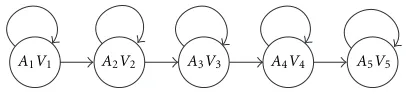
A1V1 A2V2 A3V3 A4V4 A5V5
Figure2: The state transition diagram of a left-to-right HMM.
visual features for speech recognition, especially under noisy environments, has been demonstrated by the success of re-cent AVSR systems [2]. However, problems such as the selec-tion of the optimal set of visual features, or the optimal mod-els for audio-visual integration remain challenging research topics. In this paper, we describe a set of improvements to the existing methods for visual feature selection and we focus on two models for isolated word audio-visual speech recogni-tion: the coupled hidden Markov model (CHMM) [3] and the factorial hidden Markov model (FHMM) [4], which are special cases of the dynamic Bayesian networks [5]. The structure of both models investigated in this paper describes the state synchrony of the audio and visual components of speech while maintaining their natural correlation over time. The isolated word AVSR system illustrated in Figure 1 is used to analyze the performance of the audio-visual models in-troduced in this paper. First, the audio and visual features (Section 3) are extracted from each frame of the audio-visual sequence. The sequence of visual features, which describe the mouth deformation over consecutive frames, is upsampled to match the frequency of the audio observation vectors. Fi-nally, both the factorial and the coupled HMM (Section 4) are used for audio-visual integration, and their performance for AVSR in terms of parameter complexity, computational efficiency (Section 5), and recognition accuracy (Section 6) is compared to existing models used in current AVSR systems.
2. RELATED WORK
Audio-visual speech recognition has emerged in recent years as an active field, gathering researchers in computer vision, signal and speech processing, and pattern recognition [2]. With the selection of acoustic features for speech recognition well understood [6], robust visual feature extraction and se-lection of the audio-visual integration model are the leading research areas in audio-visual speech recognition.
Visual features are often derived from the shape of the mouth [7, 8, 9, 10]. Although very popular, these methods rely exclusively on the accurate detection of the lip contours
which is often a challenging task under varying illumina-tion condiillumina-tions and rotaillumina-tions of the face. An alternative ap-proach is to obtain visual features from the transformed gray scale intensity image of the lip region. Several intensity or ap-pearance modeling techniques have been studied, including principal component analysis [9], linear discriminant analy-sis (LDA), discrete cosine transform (DCT), and maximum likelihood linear transform [2]. Methods that combine shape and appearance modeling were presented in [2, 11].
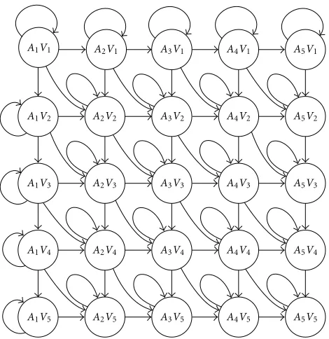
A1V1 A2V1 A3V1 A4V1 A5V1
A1V2 A2V2 A3V2 A4V2 A5V2
A1V3 A2V3 A3V3 A4V3 A5V3
A1V4 A2V4 A3V4 A4V4 A5V4
A1V5 A2V5 A3V5 A4V5 A5V5
Figure3: The state transition diagram of a product HMM.
3. VISUAL FEATURE EXTRACTION
Robust location of the facial features, specially the mouth re-gion, and the extraction of a discriminant set of visual obser-vation vectors are the two key elements of the AVSR system. The cascade algorithm for visual feature extraction used in our AVSR system consists of the following steps: face detec-tion, mouth region detecdetec-tion, lip contour extracdetec-tion, mouth region normalization and windowing, 2D-DCT and LDA co-efficient extraction. Next, we will describe the steps of the cascade algorithm in more detail.
The extraction of the visual features starts with the de-tection of the speaker’s face in the video sequence. The face detector used in our system is described in [18]. The lower half of the detected face (Figure 4a) is a natural choice for the initial estimate of the mouth region.
Next, LDA is used to assign the pixels in the mouth region to the lip and face classes. LDA transforms the pixel values from the RGB chromatic space into a one-dimensional space that best separates the two classes. The optimal linear dis-criminant space [19] is computed off-line using a set of man-ually segmented images of the lip and face regions. Figure 4b shows a binary image of the lip segmentation from the lower region of the face in Figure 4a.
The contour of the lips (Figure 4c) is obtained through the binary chain encoding method [20] followed by a smoothing operation. Figures 5a, 5b, 5c, 5d, 5e, 5f, and 5h show several successful results of the lip contour extraction. Due to the wide variety of skin and lip tones, the mouth seg-mentation and therefore the lip contour extraction may re-sult in inaccurate rere-sults (Figures 5i and 5j).
The lip contour is used to estimate the size and the ro-tation of the mouth in the image plane. Using an affine
(a) (b)
(c) (d) (e)
Figure4: (a) The lower region of the face used as an initial estimate for the mouth location, (b) binary image representing the mouth segmentation results, (c) the result of the lip contour extraction, (d) the scale and rotation normalized mouth region, (e) the result of the normalized mouth region windowing.
transform a rotation and size normalized grayscale region of the mouth (64×64 pixels) is obtained from each frame of the video sequence (Figure 4d). However, not all the pix-els in the mouth region have the same relevance for visual speech recognition. In our experiments we found that, as ex-pected, the most significant information for speech recogni-tion is contained in the pixels inside the lip contour. There-fore, we use an exponential windoww[x, y] =exp(−((x− x0)2+ (y−y0)2)/σ2),σ=12, to multiply the pixels values in the grayscale normalized mouth region. The window of size 64×64 is centered in the center of the mouth region (x0, y0). Figure 4e illustrates the result of the mouth region window-ing.
Next, the normalized and windowed mouth region is de-composed into eight blocks of height 32 and width 16, and the 2D-DCT transform is applied to each of these blocks. A set of four 2D-DCT coefficients from a window of size 2×2 in the lowest frequency in the 2D-DCT domain are extracted from each block. The resulting coefficients extracted are ar-ranged in a vector of size 32.
In the final stage of the video feature extraction cascade, the multiclass LDA [19] is applied to the vectors of 2D-DCT coefficients. For our isolated word speech recognition sys-tem, the classes of the LDA are associated to the words avail-able in the database. A set of 15 coefficients, corresponding to the most significant generalized eigenvalues of the LDA decomposition are used as visual observation vectors.
4. THE AUDIO-VISUAL MODEL
(a) (b) (c) (d) (e)
(f) (g) (h) (i) (j)
Figure5: Examples of the mouth contour extraction.
t=0, t=1, . . . t, . . . t=T−2, t=T−1 · · · ·
Backbone nodes Mixture nodes Observation nodes
Figure6: The audio-visual HMM.
terms of individual variables or factors. A DBN is speci-fied by a directed acyclic graph, which represents the condi-tional independence assumptions and the condicondi-tional prob-ability distributions of each node [23, 24]. With the DBN representation, the classification of the decision fusion mod-els can be seen in terms of independence assumptions of the transition probabilities and of the conditional likeli-hood of the observed and hidden nodes. Figure 6 sents an HMM as a DBN. The transparent squares repre-sent the hidden discrete nodes (variables), while the shaded circles represent the observed continuous nodes. Through-out this paper, we will refer to the hidden nodes condi-tioned over time as coupled or backbone nodes and to the remaining hidden nodes as mixture nodes. The variables associated with the backbone nodes represent the states of the HMM, while the values of the mixture nodes represent the mixture component associated with each of the state of the backbone nodes. The parameters of the HMM [6] are
π(i)=Pq1=i
,
bt(i)=POt|qt=i,
a(i|j)=Pqt=i|qt−1=j
,
(1)
whereqt is the state of the backbone node at timet,π(i) is
the initial state distribution for statei,a(i|j) is the state tran-sition probability from state jto statei, andbt(i) represents the probability of the observation Ot given theith state of the backbone nodes. The observation probability is generally modeled using a mixture of Gaussian components.
Introduced for audio-only speech recognition, the mul-tistream HMM a (MSHMM) became a popular model for multimodal sequences such as the audio-visual speech. In
bt(i)= S
s=1
Ms i
m=1
ws
i,mNOst,µsi,m,Usi,m
λs
, (2)
whereSrepresents the total number of streams,λs(sλs=
1, λs ≥ 0) are the stream exponents, Ost is the observa-tion vector of the sth stream at timet,Mis is the number of mixture components in stream s and state i, and µsi,m, Usi,m, wi,ms are the mean, covariance matrix, and mixture weight for thesth stream,ith state, andmth Gaussian mix-ture component, respectively. The two streams (S = 2) of the audio-visual MSHMM (AV MSHMM) model the audio and the video sequence. For the AV MSHMM, as well as for the HMM used in video-only or audio-only speech recogni-tion, all covariance matrices are assumed diagonal, and the transition probability matrix reflects the left-to-right state evolution
a(i|j)=0, ifi /∈ {j, j+ 1}. (3)
The audio and visual state synchrony imposed by the AV MSHMM can be relaxed using models that allow one hidden backbone node per stream at each timet. Figure 7 illustrates a two-stream independent HMM (IHMM) represented as a DBN. Leti = {i1, . . . , iS}be some set of states of the back-bone nodes,Nsthe number of states of the backbone nodes in streams,qtsthe state of the backbone node in streamsat timetandqt = {q1
t=0, t=1, . . . t, . . . t=T−2, t=T−1 · · ·
· · ·
· · · · · ·
Figure7: A two-stream independent HMM.
t=0, t=1, . . . t, . . . t=T−2, t=T−1 · · · ·
Figure8: The audio-visual product HMM.
IHMM are
π(i)=
s π
sis= s P
qs
1=is
, (4)
bt(i)=
s b s tis=
s P
Ost|qts=is, (5)
a(i|j)=
s a si
s|js=
s P
qs
t=is|qst−1=js
, (6)
whereπs(is) andbst(is) are the initial state distribution and the observation probability of state is in stream s, respec-tively, andas(is|js) is the state transition from statejsto state
isin streams. For the audio-visual IHMM (AV IHMM) each of the two HMMs, describing the audio or video sequence, is constrained to a left-to-right structure, and the observa-tion likelihoodbst(i) is computed using a mixture of Gaussian density functions, with diagonal covariance matrices. The AV IHMM allows for more flexibility than the AV MSHMM in modeling the state asynchrony but fails to model the natural correlation in time between the audio and visual components of speech. This is a result of the independent modeling of the transition probabilities (see (6)) and of the observation like-lihood (see (5)).
A product HMM (PHMM) can be seen as a standard HMM, where each backbone state is represented by a set of states, one for each stream [17]. The parameters of a PHMM
are
π(i)=Pq1=i
, (7)
bt(i)=POt|qt=i, (8)
a(i|j)=Pqt=i|qt−1=j
, (9)
whereOtcan be obtained through the concatenation of the observation vectors in each stream
Ot=O1
tT, . . . ,OStT T
. (10)
The observation likelihood can be computed using a Gaus-sian density or a mixture with GausGaus-sian components. The use of PHMM in AVSR is justified primarily because it allows for state asynchrony, since each of the coupled nodes can be in any combination of audio and visual states. In addition, unlike the IHMM, the PHMM preserves the natural corre-lation of the audio and visual features due the joint proba-bility modeling of both the observation likelihood (see (8)) and transition probabilities (see (9)). For the PHMM used in AVSR, denoted in this paper as the audio-visual PHMM (AV PHMM), the audio and visual state asynchrony is limited to a maximum of one state. Formally, the transition probability matrix from statej=[ja, jv] to statei=[ia, iv] is given by
a(i|j)=0 if
is∈/ js, js+ 1, s∈ {a, v},
ia−iv≥2, i=j, (11)
where indices aandvdenote the audio and video stream, respectively. In the AV PHMM described in this paper (Figure 8) the observation likelihood is computed using
bt(i)= Mi
m=1
wi,m
s
NOst,µsi,m,Usi,mλs, (12)
t=0, t=1, . . . t, . . . t=T−2, t=T−1 · · ·
· · ·
· · · · · ·
Figure9: The audio-visual factorial HMM.
4.1. The audio-visual factorial hidden Markov model
The factorial HMM (FHMM) [4] is a generalization of the HMM suitable for a large range of multimedia applications that integrate two or more streams of data. The FHMM gen-eralizes an HMM by representing the hidden state by a set of variables or factors. In other words, it uses a distributed rep-resentation of the hidden state. These factors are assumed to be independent of each other, but they all contribute to the observations, and hence become coupled indirectly due to the “explaining away” effect [23]. The elements of a factorial HMM are described as
π(i)=Pq1=i
, (13)
bt(i)=POt|qt=i, (14)
a(i|j)=
s a si
s|js=
s P
qs
t=is|qts−1=js
. (15)
It can be seen that as with the IHMM, the transition proba-bilities of the FHMM are computed using the independence assumption between the hidden states or factors in each of the HMMs (see (15)). However, as with the PHMM, the ob-servation likelihood is jointly computed from all the hidden states (see (14)). The observation likelihood can be com-puted using a continuous mixture with Gaussian compo-nents. The FHMM used in AVSR, denoted in this paper as the audio-visual FHMM (AV FHMM), has a set of modifications from the general model. In the AV FHMM used in this paper (Figure 9), the observation likelihoods are obtained from the multistream representation as described in (12). To model the causality in speech generation, the following constraint on the transition probability matrices of the AV FHMM is imposed:
asi
s|js=0, ifis∈/ js, js+ 1, (16)
wheres∈ {a, v}.
4.1.1 Training factorial HMMs
As is well known, DBNs can be trained using the expectation-maximization (EM) algorithm (see, e.g., [22]). The EM algo-rithm for the FHMM is described in Appendix A. However, this only converges to a local optimum, making the choice
of the initial parameters of the model a critical issue. In this paper, we present an efficient method for initialization us-ing a Viterbi algorithm derived for the FHMM. The Viterbi algorithm for FHMMs is described below for an utterance O1, . . . ,OT of lengthT.
(i) Initialization
δ1(i)=π(i)b1(i), (17)
ψ1(i)=0; (18)
(ii) Recursion
δt(i)=max
j
δt−1(j)a(i|j)bt(i),
ψt(i)=arg max
j
δt−1(j)a(i|j);
(19)
(iii) Termination
P∗=max
i
δT(i),
qT=arg max
i
δT(i);
(20)
(iv) Backtracking
qt=ψt+1
qt+1
, (21)
whereP∗ = maxq1,...,qTP(O1, . . . ,OT,q1, . . . ,qT), anda(i|j) is obtained using (15). Note that, as with the HMM, the Viterbi algorithm can be computed using the logarithms of the model parameters, and additions instead of multiplica-tion.
The initialization of the training algorithm iteratively up-dates the initial parameters of the model from the optimal segmentation of the hidden states. The state segmentation algorithm described in this paper reduces the complexity of the search for the optimal sequence of backbone and mixture nodes using the following steps. First, we use the Viterbi algo-rithm, as described above, to determine the optimal sequence of states for the backbone nodes. Second, we obtain the most likely assignment to the mixture nodes. Given these optimal assignments to the hidden nodes, the appropriate sets of pa-rameters are updated. For the FHMM withλs =1 and gen-eral covariance matrices the initialization of the training al-gorithm is described below.
Step 1. Let Rbe the number of training examples and let Osr,1, . . . ,Osr,Trbe the observation sequence of lengthTr
cor-responding to thesth stream of therth (1≤r ≤R) training example. First, the observation sequencesOsr,1, . . . ,Osr,Tr are uniformly segmented according to the number of states of the backbone nodesNs. Then, a new sequence of observation vectors is obtained by concatenating the observation vectors assigned to each stateis,s=1, . . . , S. For each state setiof the backbone nodes, the mixture parameters are initialized using the K-means algorithm [19] withMiclusters.
µs
where qsr,t represents the state of thetth backbone node in the sth stream of the rth observation sequence, and cr,t is the mixture component of therth observation sequence at timet.
Step3. An optimal state sequenceqr,1, . . . ,qr,Tr of the
back-bone nodes is obtained for therth observation sequence us-ing the Viterbi algorithm (see below). The mixture compo-nentcr,tis obtained as
cr,t=m=max
1,...,Mi
POr,t|qr,t=i, cr,t=m. (24)
Step4. The iterations in Steps 2, 3, and 4 are repeated un-til the difference between the observation probabilities of the training sequences at consecutive iterations falls below a con-vergence threshold.
4.1.2 Recognition using the factorial HMM
To classify a word, the log likelihood of each model is com-puted using the Viterbi algorithm described in the previous section. The parameters of the FHMM corresponding to each word in the database are obtained in the training stage us-ing clean audio signals (SNR =30 dB). In the recognition stage, the audio tracks of the testing sequences are altered by white noise with different SNR levels. The influence of the audio and visual observation streams is weighted based on the relative reliability of the audio and visual features for dif-ferent levels of the acoustic SNR. Formally, the observation likelihoods are computed using the multistream representa-tion in (12). The values of the audio and visual exponents
λs,s∈ {a, v}, corresponding to a specific acoustic SNR level
are obtained experimentally to maximize the average recog-nition rate. Figure 10 illustrates the variation of the audio-visual speech recognition rate for different values of the au-dio exponentλaand different values of SNR. Note that each
of the AVSR curves at all SNR levels reaches smooth maxi-mum levels. This is particularly important in designing ro-bust AVSR systems and allows for the exponents to be cho-sen in a relatively large range of values. Table 1 describes the
Table1: The optimal set of exponents for the audio streamλafor
the FHMM at different SNR values of the acoustic speech.
SNR (dB) 30 28 26 24 22 20 18 16 14 12 10
λa 0.8 0.8 0.7 0.6 0.6 0.3 0.2 0.1 0.1 0.1 0.0
audio exponentsλaused in our system which were derived from Figure 10. As expected, the value of the optimal audio exponents decays with the decay of the SNR levels, showing the increased reliability of the video at low acoustic SNR.
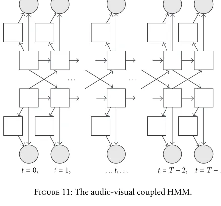
4.2. The audio-visual coupled hidden Markov model The coupled HMM (CHMM) [3] is a DBN that allows the backbone nodes to interact, and at the same time to have their own observations. In the past, CHMM have been used to model hand gestures [3], the interaction between speech and hand gestures [25], or audio-visual speech [26, 27]. Figure 11 illustrates a continuous mixture two-stream CHMM used in our audio-visual speech recognition system. The elements of the coupled HMM are described as
π(i)=
Note that in general, to decrease the complexity of the model, the dependency of a backbone node at timetis restricted to its neighbor backbone nodes at timet−1. As with the IHMM, in the CHMM the computation of the observation likelihood assumes the independence of the observation likelihoods in each stream. However, the transition probability of each cou-pled node is computed as joint probability of the set of states at previous time. With the constraint as(is|j) = as(is|js) a
CHMM is reduced to an IHMM.
For the audio-visual CHMM (AV CHMM) the observa-tion likelihoods of the audio and video streams are computed using a mixture of Gaussians with diagonal covariance ma-trices, and the transition probability matrix is constrained to reflect the natural audio-visual speech dependencies
0 0.1 0.2 0.3 0.4 0.5 0.6 0.7 0.8 0.9 1
t=0, t=1, . . . t, . . . t=T−2, t=T−1 · · · ·
Figure11: The audio-visual coupled HMM.
t=0, t=1, t=2, t=3, · · · t=T−2, t=T−1 · · ·
· · · Video
Audio
Figure12: The Boltzmann zipper used in audio-visual integration.
Boltzmann zipper can address the problem of “fast” (audio) and “slow” (visual) observation vector integration.
4.2.1 Training the coupled HMM
In the past, several training techniques for the CHMM were proposed including the Monte Carlo sampling method and the N-head dynamic programming method [3, 26]. The CHMM in this paper is trained using EM (Appendix B) which makes the choice of robust initial parameters very im-portant. In this section we describe an efficient initialization method of the CHMM parameters, which is similar to the initialization of the FHMM parameters described previously. The initialization of the training algorithm for the CHMM is described by the following steps:
Step1. GivenRtraining examples, the observation sequence of length Tr corresponding to the rth example (1 ≤ r ≤ R) and sth stream, Osr,1, . . . ,Osr,Tr, is uniformly segmented
according to the number of states of the backbone nodes
Ns. Hence an initial state sequence for the backbone nodes
qs
r,1, . . . , qsr,t, . . . , qsr,Tr is obtained for each data streams. For
each stateiin streamsthe mixture segmentation of the data assigned to it is obtained using the K-means algorithm [19] withMisclusters. Consequently the mixture componentscsr,t
for therth observation sequence at timetand streamsis ob-tained.
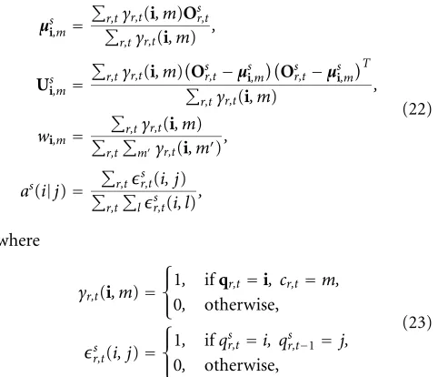
Step2. The new parameters of the model are estimated from the segmented data
µs i,m=
r,tγr,ts (i, m)Osr,t
r,tγr,ts (i, m) ,
Usi,m=
r,tγr,ts (i, m)Osr,t−µsi,m
Osr,t−µs i,m
T
r,tγsr,t(i, m) ,
ws i,m=
r,tγr,ts (i, m)
r,tmγsr,t(i, m),
as(i|j)=
r,tsr,t(i,j)
r,tjsr,t(i,j) ,
(29)
where
γs
r,t(i, m)=
1, ifqsr,t=i, cs r,t=m,
0, otherwise,
sr,t(i,j)=
1, ifqsr,t=i,qr,t−1=j, 0, otherwise,
(30)
wherecsr,tis the mixture component for thesth stream of the
rth observation sequence at timet.
Step 3. An optimal state sequence of the backbone nodes qr,1, . . . ,qr,Tr is obtained using the Viterbi algorithm for the
CHMM [29]. The steps of the Viterbi segmentation for the CHMM are described by (17), (18), (19), (20), and (21), where the initial state probabilityπ(i), the observation like-lihoodb(i) and transition probabilitiesa(i|j) are computed using (25), (26), and (27), respectively. The mixture compo-nentscsr,tare obtained using
cs
r,t=m=max1,...,Ms iP
Osr,t|qsr,t=i, cs
r,t=m. (31)
Step4. The iterations in Steps 2, 3, and 4 are repeated un-til the difference between the observation probabilities of the training sequences at consecutive iterations falls below a con-vergence threshold.
4.2.2 Recognition using the coupled HMM
The isolated word recognition is carried out via the Viterbi algorithm for CHMM, where the observation probability for each observation conditional likelihood is modified to han-dle different levels of noise
˜
bs
tis=btOts|qst=isλs, (32)
Table2: The optimal set of exponents for the audio streamλa at
different SNR values of the acoustic speech for the CHMM.
SNR (dB) 30 28 26 24 22 20 18 16 14 12 10
λa 0.9 0.7 0.8 0.7 0.5 0.4 0.3 0.2 0.2 0.2 0.1
the audio sequences were perturbed by white noise. The aver-age audio-only, video-only, and CHMM-based audio-visual recognition rates for different levels of SNR are shown in Figure 14.
5. MODEL COMPLEXITY ANALYSIS
Together with the recognition accuracy, the number of pa-rameters of the model and the computational complexity re-quired by the recognition process are very important in the analysis of a model. Models with a small number of parame-ters produce better estimates for the same amount of training data. Tables 3, 4, 5, and 6 describe the size of the parameter space and the computational complexity required for recog-nition using the PHMM, IHMM, FHMM, and CHMM. We consider both the general case as well as the specific mod-els used in AVSR (i.e., AV PHMM, AV IHMM, AV FHMM, and AV CHMM) which include the use of diagonal covari-ance matrices, and sparse transition probability matrices as described in Section 4. In addition to the notations intro-duced in the previous section, the size of the observation vec-tor in modalitysis denoted byVs. For simplification, for the IHMM and CHMM, we consider that all the mixture nodes in streamshave the same number of componentsMs, inde-pendent of the state of the parent backbone nodes. For the PHMM and FHMM we assume that all state sets have the same number of mixture componentsM.
In terms of the space required by the parameters of the models, we count the elements of the transition probability matrices (A), the mean vectors (µ), covariance matrices (U), and the weighting coefficients (w) per HMM word. From Tables 3 and 6 we see that the IHMM and CHMM as well as the AV IHMM and AV CHMM, require the same num-ber of parameters for µ,U, andw. This is due to the fact that in these models, the probability of the observation vec-torOstin streamsat timetdepends only on its private mix-ture and backbone node. Due to the coupling of the back-bone nodes, the space required by theAparameters of the CHMM and AV CHMM is larger than that for the IHMM and AV IHMM, respectively. However, ifVsNs, the space required by theAparameters is negligible compared toµ,U andw, making the AV CHMM and AV IHMM very similar from the point of view of the parameter space requirements. The joint dependency of the observation vector Ot on all backbone nodes at timetfor the PHMM, FHMM increases significantly the number of parameters of these models com-pared to the IHMM and CHMM (Tables 4 and 5). Note that the left-to-right topology of each HMM in an AV FHMM (see (16)) does not reduce the number of audio-visual state combinations which remains of the order of2s=1Ns. On the
Table3: The number of parameters and running time needed for independent HMMs, and for the specific model used in AVSR.
Space IHMM AV IHMM
A O(sN2
s) O(2s=1Ns)
µ sNsMsVs 2s=1NsMsVs
U sNsMsVs2 2s=1NsMsVs
w sNsMs 2s=1NsMs
Time IHMM AV IHMM
Viterbi O(sNs2) O(2s=1Ns)
Table4: The number of parameters and running time needed for the product HMM, and for the specific model used in AVSR.
Space PHMM AV PHMM
A O(sN2
s) O(2s=1Ns)
µ (sNs)M(sVs) O(2s=1NsM 2
s=1Vs)
U (sNs)M(sVs)2 O(2
s=1NsM
2
s=1Vs)
w (sNs)M O(2s=1NsM)
Time PHMM AV PHMM
Viterbi O(sN2
s) O(2s=1Ns)
Table5: The number of parameters and running time needed for the factorial HMM, and for the specific model used in AVSR.
Space FHMM AV FHMM
A O(sN2
s) O(2s=1Ns)
µ (sNs)M(sVs) 2s=1( 2
s=1Ns)MVs
U (sNs)M(sVs)2 2s=1( 2
s=1Ns)MVs
w (sNs)M (2s=1Ns)M
Time FHMM AV FHMM
Viterbi O(sNs2) O(2s=1Ns2)
other hand, the sparse transition probability matrix of the AV PHMM (see (11)) only allows a number of audio-visual states of the order of √2s=1Ns. This reduces the parame-ter space of the AV PHMM compared to the AV FHMM while still remaining more complex than the AV IHMM or AV CHMM.
0 0.1 0.2 0.3 0.4 0.5 0.6 0.7 0.8 0.9 1
10 12 14 16 18 20 22 24 26 28 30 Acoustic SNR (dB)
0 10 20 30 40 50 60 70 80 90 100
R
ec
o
gnition
rat
e
(%)
Audio-visual Video Audio
Figure14: Comparison of the recognition rate of the audio-only, video-only and CHMM-based audio-visual speech recognition.
Table6: The number of parameters and running time needed for the coupled HMM, and for the specific model used in AVSR.
Space CHMM AV CHMM
A O((sNs)(sNs)) O(2s=1Ns)
µ sNsMsVs 2s=1NsMsVs
U sNsMsVs2 2s=1NsMsVs
w sNsMs 2s=1NsMs
Time CHMM AV CHMM
Viterbi O(sNs2) O(2s=1Ns)
joint dependency of the observation node from all the back-bone nodes in the same time slicetfor the AV FHMM and AV PHMM, or the joint state transition probabilities from all the backbone nodes at timet−1 for the AV PHMM and AV CHMM increases significantly the complexity of the Viterbi algorithm for these models. Unlike the AV FHMM, in the AV PHMM and AV CHMM the total number of possible audio-visual states is restricted by the sparse transition probabil-ity matrix (see (11) and (28)) reducing the stated decoding complexity of these models. Note that withMs≈Ns, which
is the case for our experiments, orMs Ns, which is the case in large vocabulary applications, the dominant role in the complexity required by the recognition process is played by the number of calls to the exponential function needed per time step to evaluate the observation likelihoods. This num-ber equals the total numnum-ber of elements of mixture weights shown in the row labeled w. Therefore, we can conclude that in terms of both the size of the parameter space and the recognition complexity, the AV CHMM and AV IHMM
Table7: A comparison of the video-only speech recognition rates for different video feature extraction techniques.
Video features Recognition rate
1D DCT, LDA 43.06%
Window, 1D DCT, LDA 52.50%
2D DCT blocks, LDA 64.17%
Window, 2D DCT blocks, LDA 66.94%
compare closely and outperform the AV PHMM, especially the AV FHMM. However, unlike the AV IHMM, the cou-pling of the backbone nodes in the AV CHMM can model the correlation of the audio-visual components of speech. In the next section, we will complete the analysis of the above models with the experimental results in audio-visual speech recognition.
6. EXPERIMENTAL RESULTS
We tested the speaker dependent isolated word audio vi-sual recognition system on the CMU database [18]. Each word in the database is repeated ten times by each of the ten speakers in the database. For each speaker, nine exam-ples of each word were used for training and the remaining example was used for testing. In our experiments we com-pared the accuracy of the only, video-only and audio-visual speech recognition systems using the AV MSHMM, AV CHMM, AV FHMM, AV PHMM, and AV IHMM de-scribed in Section 4. For each of the audio-only and video-only recognition tasks, we model the observation sequences using a left-to-right HMM with five states, three Gaussian mixtures per state and diagonal covariance matrices. In the audio-only and all audio-visual speech recognition experi-ments, the audio sequences used in training are captured in clean acoustic conditions and the audio track of the testing sequences was altered by white noise at various SNR levels from 30 dB (clean) to 12 dB. The audio observation vectors consist of 13 MFC coefficients [6], extracted from overlap-ping frames of 20 ms. The visual observations are obtained using the cascade algorithm described in Section 3.
Table 7 shows the effect of the mouth region window-ing and 2D-DCT coefficients extraction (window, 2D-DCT, LDA) on the visual-only recognition rate. It can be seen that the cascade algorithm that uses 2D-DCT coefficients extracted from eight non overlapping blocks of the mouth region followed by LDA (2D-DCT, LDA) outperforms the system that uses 32 1D-DCT coefficients extracted from the mouth region followed by LDA with the same number of co-efficients (1D-DCT, LDA). In addition the use of mouth re-gion windowing in the cascade algorithm (window, 1D-DCT, LDA or window, 2D-DCT, LDA) increases the recognition rate of the system without data windowing (1D-DCT, LDA and 2D-DCT, LDA, respectively).
Table8: A comparison of the speech recognition rate at different levels of acoustic SNR using an HMM for video-only features (V HMM), an HMM for audio-only features (A HMM), an MSHMM for audio-visual features (AV MSHMM), the independent audio-visual HMM (AV IHMM), the product audio-visual HMM (AV PHMM), the factorial audio-visual HMM (AV FHMM) and the coupled audio-visual HMM (AV CHMM).
SNR (dB) 30 28 26 24 22 20 18 16 14 12 10
V HMM (%) 66.9 66.9 66.9 66.9 66.9 66.9 66.9 66.9 66.9 66.9 66.9
A HMM (%) 96.9 89.5 85.0 79.2 69.2 60.8 50.0 38.3 28.0 20.8 15.0
AV MSHMM (%) 98.6 93.5 90.5 87.0 84.3 79.2 74.6 72.7 70.3 68.1 67.8
AV IHMM (%) 97.6 93.0 90.5 87.8 84.0 78.9 76.2 71.6 69.2 67.6 67.6
AV PHMM (%) 97.8 91.6 89.2 86.8 83.5 78.9 74.9 73.0 71.1 68.6 67.3
AV FHMM (%) 97.8 91.6 88.9 86.5 82.7 78.6 74.9 72.7 69.5 67.8 66.8
AV CHMM (%) 98.1 94.1 91.9 88.9 86.8 81.9 76.8 74.1 71.1 68.9 65.7
three Gaussian density functions, with diagonal covariance matrices. We trained all AV models using equal stream ex-ponents (λa = λv = 1). In testing, the value of the stream
exponents were chosen to maximize the average recognition rate for each value of the acoustic SNR. Our experimen-tal results shown in Table 8 indicate that the CHMM-based audio-visual speech recognition system performs best over-all, achieving the highest recognition rates in a wide range of SNR from 12 dB to 30 dB. As expected, all the audio-visual systems outperform significantly the audio-only recognition rate in noisy conditions, reaching about 50% reduction in the word error rate at SNR=10 dB. Note that at SNR=10 dB the AVSR recognition rate is practically bounded by the video-only recognition.
7. CONCLUSIONS
This paper studies the use of two types of dynamic Bayesian networks, the factorial and the coupled HMM, and com-pares their performances with existing models for audio-visual speech recognition. Both the FHMM and CHMM are generalizations of the HMM suitable for a large variety of multimedia applications that involve two or more streams of data. The parameters of the CHMM and FHMM, as special cases of DBN, can be trained using EM. However, EM is a local optimization algorithm that makes the choice of the initial parameters a critical issue. In this paper, we present an efficient method for the parameter initialization, using a Viterbi algorithm derived for each of the two models. For AVSR, the CHMM and the FHMM with two streams, one for audio and one for visual observation sequences, are par-ticularly interesting. Both models allow for audio and visual state asynchrony, while still preserving the natural correla-tion of the audio and visual observacorrela-tions over time. With the FHMM, the audio and visual states are independent of each other, but they jointly model the likelihood of the audio-visual observation vector, and hence become correlated indi-rectly. On the other hand, with the CHMM, the likelihoods of the audio and visual observation vectors are modeled
independently of each other, but each of the audio and vi-sual states are conditioned jointly by the previous set of au-dio and visual states. The performance of the FHMM and the CHMM for speaker dependent isolated word AVSR was com-pared with existing models such as the multistream HMM, the independent HMM and the product HMM. The coupled HMM-based system outperforms all the other models at all SNR levels from 12 dB to 30 dB. The lower performance of the FHMM can be an effect of the large number of parame-ters required by this model, and the relatively limited amount of data in our experiments. In contrast, the efficient struc-ture of the CHMM requires a small number of parameters, comparable to the independent HMM, without reducing the flexibility of the model. The best recognition accuracy in our experiments, the low parameter space, and the ability to ex-ploit parallel computation make the CHMM a very attractive choice for audio visual integration. Our preliminary experi-mental results [30] show that the CHMM is a viable tool for speaker independent audio-visual continuous speech recog-nition.
APPENDICES
A. THE EM ALGORITHM FOR FHMM
The EM algorithm for the multistream FHMM (see (12)) withλs=1 and general covariance matrices is described by the following steps.
E Step. The forward probability, defined as αt(i) =
P(O1, . . . ,Ot, qt =i), and the backward probabilityβt(i)=
P(Ot+1, . . . ,OT|qt = i) are computed as follows. Starting with the initial conditions
α1(i)=π(i)b1(i), (A.1)
the forward probabilities are computed recursively from
αt(i)=bt(i)
j
fort=2,3, . . . , T. Similarly, from the initial conditions
βT(i)=1, (A.3) the backward probabilities are computed recursively from
βt(j)=
i
bt+1(i)a(i|j)βt+1(i) (A.4)
fort=T−1, T−2, . . . ,1. The transition probabilitya(i|j) is computed according to (15). The probability of the rth observation sequenceOr of lengthTr, is computed asPr =
αr,Tr(N1, . . . , NS)= βr,1(1, . . . ,1) whereαr,t, andβr,t are the
forward and backward variables for therth observation se-quence.
M Step. The forward and backward probabilities obtained in
the E step are then used to re-estimate the state parameters using
The state transition probabilities can be estimated using
˜ where vectorsiandjin (A.7) can be any state vectors such thatis=iandjs= j, respectively.
B. THE EM ALGORITHM FOR CHMM
The EM algorithm for the CHMM is described by the follow-ing steps.
E Step. The forward probability and backward
probabil-ity and the observation probabilprobabil-ity Pr are computed as in Appendix A, where the initial state probabilityπ(i), the ob-servation probability bt(i), and the transition probability
a(i|j) are computed as in (25), (26), and (27).
M Step. The forward and backward probabilities obtained in
the E step are used to re-estimate the state parameters as fol-lows:
The state transition probabilities can be estimated using
˜
[1] H. McGurk and J. MacDonald, “Hearing lips and seeing
voices,”Nature, vol. 264, no. 5588, pp. 746–748, 1976. [2] C. Neti, G. Potamianos, J. Luettin, et al., “Audio visual speech
recognition, Final workshop 2000 report,” Tech. Rep., Cen-ter for Language and Speech Processing, The Johns Hopkins University, Baltimore, Md, USA, 2000.
[3] M. Brand, N. Oliver, and A. Pentland, “Coupled hidden
Markov models for complex action recognition,” in Proc.
IEEE International Conference on Computer Vision and Pattern Recognition, pp. 994–999, San Juan, Puerto Rico, June 1997. [4] Z. Ghahramani and M. I. Jordan, “Factorial hidden Markov
models,” inProc. Conf. Advances in Neural Information Pro-cessing Systems, D. S. Touretzky, M. C. Mozer, and M. E. Has-selmo, Eds., vol. 8, pp. 472–478, MIT Press, Cambridge, Mass, USA, 1995.
[5] T. Dean and K. Kanazawa, “A model for reasoning about per-sistence and causation,”Artificial Intelligence, vol. 93, no. 1-2, pp. 1–27, 1989.
[6] L. Rabiner and B.-H. Juang, Fundamentals of Speech Recogni-tion, Prentice-Hall, Englewood Cliffs, NJ, USA, 1993. [7] J. Luettin, N. Thacker, and S. Beet, “Speechreading using
shape and intensity information,” inProc. the 4th IEEE In-ternational Conf. on Spoken Language Processing, vol. 1, pp. 58–61, Philadelphia, Pa, USA, 1996.
[8] T. Chen, “Audiovisual speech processing,” IEEE Signal Pro-cessing Magazine, vol. 18, pp. 9–21, January 2001.
[9] C. Bregler and S. Omohundro, “Nonlinear manifold learn-ing for visual speech recognition,” inProc. IEEE International Conf. on Computer Vision, pp. 494–499, Boston, Mass, USA, 1995.
[10] R. Kober, U. Harz, and J. Schiffers, “Fusion of visual
and acoustic signals for command-word recognition,” in
Proc. IEEE Int. Conf. Acoustics, Speech, Signal Processing, pp. 1495–1497, Munich, Germany, April 1997.
[12] A. Adjoudani and C. Benoˆıt, “Audio-visual speech recogni-tion compared across two architectures,” inEuropean Con-ference on Speech Communication and Technology, pp. 1563– 1566, Madrid, Spain, 1995.
[13] G. Potamianos, J. Luettin, and C. Neti, “Hierarchical dis-criminant features for audio-visual LVCSR,” inProc. IEEE Int. Conf. Acoustics, Speech, Signal Processing, pp. 165–168, Salt Lake City, Utah, USA, May 2001.
[14] J. Luettin, G. Potamianos, and C. Neti, “Asynchronous stream modeling for large vocabulary audio-visual speech recogni-tion,” inProc. IEEE Int. Conf. Acoustics, Speech, Signal Process-ing, pp. 169–172, Salt Lake City, Utah, USA, 2001.
[15] M. J. Tomlinson, M. J. Russell, and N. M. Brooke, “Integrating audio and visual information to provide highly robust speech recognition,” inProc. IEEE Int. Conf. Acoustics, Speech, Signal Processing, pp. 821–824, Atlanta, Ga, USA, May 1996. [16] Y. Zhang, S. Levinson, and T. Huang, “Speaker independent
audio-visual speech recognition,” inIEEE International Con-ference on Multimedia and Expo, vol. 2, pp. 1073–1076, New York, NY, USA, 2000.
[17] G. Gravier, G. Potamianos, and C. Neti, “Asynchrony model-ing for audio-visual speech recognition,” inProc. Human Lan-guage Technology Conference, San Diego, Calif, USA, March 2002.
[18] Advanced Multimedia Processing Lab, http://amp.ece.
cmu.edu/projects/AudioVisualSpeechProcessing/, Carnegie Mellon University, Pittsburgh, Pa, USA.
[19] R. O. Duda, P. E. Hart, and D. G. Stork,Pattern Classification, John Wiley & Sons, New York, NY, USA, 2nd edition, 2000. [20] K. R. Castleman,Digital Image Processing, Prentice-Hall,
En-glewood Cliffs, NJ, USA, 1996.
[21] U. Kjaerulff, “A computational scheme for reasoning in dy-namic probabilistic networks,” inProc. the 8th International Conference on Uncertainty in Artificial Intelligence, pp. 121– 129, Stanford, Calif, USA, 1992.
[22] Z. Ghahramani, “Learning dynamic Bayesian networks,” in
Adaptive Processing of Sequences and Data Structures, C. Giles and M. Gori, Eds., Lecture Notes in Artificial Intelligence, pp. 168–197, Springer-Verlag, Berlin, Germany, 1998.
[23] J. Pearl,Probabilistic Reasoning in Intelligent Systems: Networks of Plausible Inference, Morgan Kaufmann Publishers, San Ma-teo, Calif, USA, 1988.
[24] F. V. Jensen,Bayesian Networks and Decision Graphs, Springer-Verlag, New York, USA, 2001.
[25] V. Pavlovic,Dynamic Bayesian networks for information fusion with applications to human-computer interfaces, Ph.D. thesis, University of Illinois, Urbana-Champaign, Ill, USA, 1999. [26] S. Chu and T. Huang, “Bimodal speech recognition using
coupled hidden Markov models,” inProc. IEEE International Conf. on Spoken Language Processing, vol. 2, pp. 747–750, Bei-jing, China, 2000.
[27] S. Chu and T. Huang, “Audio-visual speech modeling
using coupled hidden Markov models,” in Proc. IEEE
Int. Conf. Acoustics, Speech, Signal Processing, pp. 2009–2012, Orlando, Fla, USA, May 2002.
[28] M. E. Hennecke, D. G. Stork, and K. V. Prasad, “Visionary speech: Looking ahead to practical speechreading systems,” in
Speechreading by Humans and Machines: Models, Systems and Applications, D. G. Stork and M. E. Hennecke, Eds., vol. 150 of
NATO ASI Series F: Computer and Systems Sciences, pp. 331– 349, Springer-Verlag, Berlin, Germany, 1996.
[29] A. Nefian, L. Liang, X. Pi, X. Liu, C. Mao, and K. Murphy, “A coupled HMM for audio-visual speech recognition,” in
Proc. IEEE Int. Conf. Acoustics, Speech, Signal Processing, pp. 2013–2016, Orlando, Fla, USA, May 2002.
[30] L. Liang, X. Liu, Y. Zhao, X. Pi, and A. Nefian, “Speaker in-dependent audio-visual continuous speech recognition,” in
IEEE International Conference on Multimedia and Expo, Lau-sanne, Switzerland, August 2002.
Ara V. Nefianis a Senior Researcher at In-tel Corporation, Microprocessor Research Labs in Santa Clara, California, USA. Ara received the engineering Diploma degree in electrical engineering in 1994 from the “Po-litehnica” University of Bucharest, Roma-nia. In 1995, he received the MSEE degree and in 1999, the Ph.D. degree, all in electri-cal engineering from Georgia Tech, Atlanta. Current research interests include the study
of graphical models for face and gesture recognition and audio-visual signal processing.
Luhong Liangis a Researcher at Intel China Research Center in Beijing. He received the Bachelor degree in 1997 and the Ph.D. de-gree in 2001, all in computer science from Tsinghua University in Beijing. His research interests include face detection and recog-nition, audio-visual signal process and bio-metrics.
Xiaobo Piis a Researcher at Intel China Re-search Center in Beijing. Xiaobo received the Bachelor degree in electronic engineer-ing in 1991 from the University of Elec-tronic Science and Technology of China. In 1994, he received the Master degree in elec-tronic engineering from Beijing Institute of Technology and in 1997, the Ph.D. degree in acoustics from Institute of Acoustics, Chi-nese Academy of Sciences. Current research
interests include speech recognition and audio-visual signal pro-cessing.
Xiaoxing Liureceived his M.S. in computer science from Fudan University. He joined Intel China Research Center in 1999. His re-search interests include speech recognition, speaker identification, speech analysis, and stochastic modeling.