DOI: 10.1534/genetics.106.063305
Inference of Bacterial Microevolution Using Multilocus Sequence Data
Xavier Didelot and Daniel Falush
1Department of Statistics, University of Oxford, Oxford OX1 3SY, United Kingdom Manuscript received July 11, 2006
Accepted for publication November 19, 2006
ABSTRACT
We describe a model-based method for using multilocus sequence data to infer the clonal relationships of bacteria and the chromosomal position of homologous recombination events that disrupt a clonal pattern of inheritance. The key assumption of our model is that recombination events introduce a constant rate of substitutions to a contiguous region of sequence. The method is applicable both to multilocus sequence typing (MLST) data from a few loci and to alignments of multiple bacterial genomes. It can be used to decide whether a subset of isolates share common ancestry, to estimate the age of the common ancestor, and hence to address a variety of epidemiological and ecological questions that hinge on the pattern of bacterial spread. It should also be useful in associating particular genetic events with the changes in phenotype that they cause. We show that the model outperforms existing methods of subdividing recombinogenic bacteria using MLST data and provide examples from Salmonella and Bacillus. The software used in this article, ClonalFrame, is available from http://bacteria.stats.ox.ac.uk/.
B
ACTERIA reproduce clonally but their genomes evolve by a variety of mechanisms, including point mutation, genome rearrangement, deletion, duplica-tion, bacteriophage lysogeny, gene degradaduplica-tion, trans-position, slippage mutation in DNA sequence repeats, and homologous and nonhomologous recombination (Maynard Smith et al. 1993; Feil et al. 1999, 2000; Lawrence and Hendrickson 2003). Recombination can occur when bacterial DNA enters the host cell via conjugation (which requires cell-to-cell contact between a donor and a receiver), transformation (uptake of naked DNA that remains from the lysis of another cell), or transduction (which involves packing of host DNA in a phage and release in the receiver).The variety of evolutionary mechanisms by which bacteria evolve can pose problems when attempting to infer relationships between strains. Clonal relationships can be represented by a genealogy, which is a tree where each leaf is a member of the sample and each internal node is the most recent common ancestor of the de-scendant strains. Each node is associated with a time before the present when that ancestor divided. Many methods for inferring these relationships rely on DNA sequence differences. Point mutations happen approx-imately randomly and independently and thus, in the absence of other processes, would allow accurate recon-struction of clonal relationships using standard phylo-genetic methods (Felsenstein1989; Swofford2002; Drummond and Rambaut 2003). However, even in ‘‘housekeeping genes’’ that are required for metabolic
function, so that gross changes in sequence such as insertions or deletions are likely to be lethal and there-fore rarely observed, homologous recombination with other bacteria from the same population can change several nucleotides at once (Milkmanand Crawford 1983). These events are overweighted by nucleotide-based phylogenetic methods in comparison to point mu-tations, which can lead to inaccurate genealogies being inferred (Schierupand Hein2000).
The necessity to account for recombination as well as point mutation in genealogical inference has led to the development of sequencing strategies such as multi-locus sequence typing (MLST), which involves sequenc-ing a handful (typically seven) of fragments from housekeeping genes that are each sufficiently far apart on the chromosome of the type strain that it would be unlikely for more than one of them to be affected by a single recombination event (Maidenet al.1998). It has also led to the use of allele designations for each unique sequence at each locus rather than the sequence itself. Alleles are considered to be equally distinct from each other whether they differ at one nucleotide position or at many with the consequence that recombination and mutation events are given similar weight in analysis. A variety of methods have been adapted, and new ones such as BURST have been developed, to analyze genetic relationships using allele designations ( Jolley et al. 2001; Feilet al.2004; Sprattet al.2004).
Allele-based methods have important limitations. Al-leles that differ at one or two nucleotides can provide evidence for a higher degree of relatedness for the strains that carry them than alleles that differ by many. For example, if recombination were rare, and a strain differed from a second one by one or two nucleotide 1Corresponding author:Peter Medawar Bldg. for Pathogen Research,
S. Parks Rd., Oxford OX1 3SY, United Kingdom. E-mail: [email protected]
differences at six of seven loci and by many nucleotides at the seventh one then the two strains would be clas-sified as unrelated by allele-based methods despite the clear evidence for a relatively recent common ancestor provided by the six similar loci. Additionally, variation in relatedness within each sequence fragment is ignored. A half fragment of identical sequence provides evidence of relatedness even if the other half contains several nucleotide differences because this spatial pattern will most likely have been caused by a homologous recom-bination event whose boundary occurred at the middle of the fragment. Allele-based methods are thus more suited to exploratory data analysis than to fine statistical inference. Ultimately, we are interested in patterns of relatedness for entire bacterial genomes and therefore would like to dispense with arbitrary boundaries be-tween loci and instead infer the beginning and end points of each homologous recombination event.
Here we describe a statistical approach for inferring bacterial clonal relationships on the basis of DNA se-quences that accounts for both point mutation and homologous recombination. In bacteria, each recom-bination event affects a contiguous region of sequence, but leaves the remainder of the circular chromosome unchanged. In the language of eukaryotic geneticists, we therefore need to model gene conversion-like events, but not crossovers. Our method estimates the extent of the clonal frame for each branch of the genealogy, which is the subset of the genome that has not under-gone recombination (Milkmanand Bridges1990). Our approach is model based in the sense that it attempts to infer the parameters and events in the evolutionary process that led to the observed pattern of DNA se-quence variation. However, our method does not at-tempt to model the origin of the DNA imported in homologous recombination events, instead assuming that imported stretches differ from the sequence they replace at a constant proportion of nucleotides,n.n is estimated from the data but does not have a straight-forward biological interpretation.
We do not attempt to model the origin of imports for two reasons. First, a full description of the ancestral relationships of all the DNA in a sample, the ancestral recombination graph (ARG), is extremely complex (Griffiths and Marjoram 1996). This complexity makes it computationally challenging to perform in-ference of the ARG even for modestly sized data sets in which the sample can be assumed to come from a closed, homogenous population in which recombina-tion takes place at a uniform rate between all pairs of strains (McVeanand Cardin 2005). Second, bacteria are often more promiscuous than eukaryotes, occasion-ally importing DNA from different species (e.g., Dingle
et al.2005) or even genera (Ochmanet al.2000), making the standard assumption of a closed, homogeneous pop-ulation particularly unrealistic. Ignoring interpopula-tion events is problematic even if they are rare because
these events can be responsible for a large number of nucleotide differences. Our method avoids both of these problems. However, because it does not look for potential sources of descent for each stretch of DNA, it tends to underestimate the number of recombina-tion events that have taken place (seeresultsbelow). Nevertheless, it is still able to infer genealogies more accurately than existing methods, with an algorithm that is fast enough to be applied to multiple bacterial genomes.
We perform inference in a Bayesian framework, which means that we need to specify a prior for the alogical process that defines the probability of any gene-alogy before observing the data. We assume a standard neutral coalescent model (Kingman 1982), which is equivalent to assuming that the bacteria in the sample come from a constant-sized population in which each bacterium is equally likely to reproduce, irrespective of its previous history. More details about the coalescent can be found, for example, in Donnellyand Tavare´ (1995). A coalescent prior has the advantage of tracta-bility and simplicity. However, it has been shown that for many bacterial populations, there is an excess of isolates with identical allelic profiles, in comparison to neutral expectations (Fraser et al. 2005; Jolley et al. 2005). Since bacteria do not disperse at each replication, dif-ferent growth conditions in difdif-ferent physical locations could introduce local correlations in the genealogy. The geographical and temporal extent of these correlations has not been established for any bacterial species and other factors such as selection and demography can also cause deviations from neutral expectation. These devia-tions might introduce biases in the genealogy produced by our method. Fortunately new genotyping technolo-gies will allow population variation to be surveyed at a genomic scale. Such data have the potential to provide a great deal of information on the shape of the genealogy, which reduces the importance of the prior and will ultimately reveal the causes of the deviations from neutrality that have been observed.
MODEL AND METHODS
We now provide a more detailed description of our modeling assumptions and the algorithms used to per-form inference. The mathematical symbols used and their meanings are summarized in Table 1.
Model: We perform statistical inference assuming
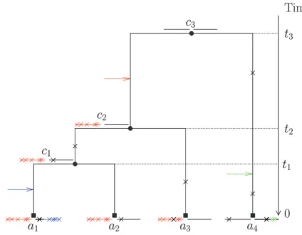
that the clonal genealogy and the sequences on each node have been generated by the probabilistic model described in this section and summarized in Figure 1. Lett1,. . .,tN1specify the times before the present at
which branching takes place in the genealogy, witht1,
t2 , . . . , tN1 and let t0 ¼0. The assumption of a
coalescent prior means that for alli2[1,. . .,N1], the difference ti ti1 is exponentially distributed with
entire genealogy,T, is equal to the product of probabil-ity of allN1 branching events,
PðT Þ ¼ Y
N1
i¼1
exp N 11i
2
ðtiti1Þ
: ð1Þ
Each sequence is assumed to consist ofbblocks of size (s1,. . .,sb), with
P
i2½1;...;bsi¼L. Each site of the se-quence at the topmost node of the tree is equally likely to be one of the four bases A, C, G, and T. The sequence associated with each daughter node is generated by the combined effects of recombination and mutation.
Re-combination happens between each node as a Poisson process of rateR/2, so that for a branch of lengthl, the total number of recombination events is Poisson dis-tributed with mean Rl/2. Each recombination event affects a contiguous stretch of the sequence of the daughter node. Only a small proportion of the chro-mosome may be available in the alignment and we model only events that affect this subset while assuming that events occur uniformly on the whole chromosome. To do this, we make the simplifying assumptions that blocks are distant enough from each other that each recombination event affects one and only one block and that recombination events are equally likely to start at any site on the genome. The total length of a recombi-nation event is assumed to be geometrically distributed with mean d. For any given recombination event that affects a given block, the probability that it starts at any nucleotide in the block except for the first is identical and is denotedu. The probability that the observed be-ginning of the event is at the first nucleotide of a block is higher and equal to
u9¼X
‘
i¼0
uPðd.iÞwithdGeomðd1Þ ð2Þ
¼uX ‘
i¼0
ð1d1Þi ¼ud: ð3Þ
Summing over all possible sites, we get
u¼ 1
bd1Lb and u9¼
d
bd1Lb: ð4Þ TABLE 1
Symbols used
Symbol Description
Data
A Aligned sequence data N Number of sequences L Total length of the sequences b Number of blocks in the alignment {si}i¼1,. . .,b Size of theith block
Model parameters
T Genealogy
R Locations of recombination events associated with the branches of the genealogy
C Ancestral sequences for the internal nodes of the genealogy
M Model parameters:n,R,d,u
u/2 Rate of mutation on the branches of the genealogy R/2 Rate of recombination on the branches of the genealogy n Rate of nucleotide differences in the recombined stretches
d Mean of the exponential distribution modeling the length of recombinant segments {ti}i¼1,. . .,N1 Age of theith coalescent event (looking back in time)
u Probability that a specific recombination event starts at any given site within a block u9 Probability that a specific recombination event starts at the beginning of a given block
a(l) Parameter of the exponential distribution modeling the length of imported regions for a branch of lengthl b(l) Parameter of the exponential distribution modeling the length of nonimported regions for a branch of lengthl
Figure1.—Illustration of the model. Two blocks (horizon-tal lines) evolve by point mutation (black crosses) and recom-bination from an unmodeled origin (colored arrows, inducing the substitutions marked by colored crosses).A ¼ fa1;a2;a3;a4g
corresponds to the observed sequences andC ¼ fc1;c2;c3g
Within the recombined regions (which are affected by at least one recombination), the daughter sequence is altered with constant raten. Within the nonrecom-bined regions the daughter sequence at each nucleo-tide is altered with probabilityul/2Lon the branches of the genealogy. Altered nucleotides are replaced accord-ing to the model of Jukesand Cantor(1969), where all substitutions are equally likely.
Inference: Given the dataA, which consist of theN
sequences at the leaves of the genealogy, we wish to infer the genealogy,T; the sequences at each of the internal nodes, C; the position of the recombined regions in each of the branches of the genealogy,R; and the four model parametersM ¼ ðn;R;d;uÞ. In formal terms, we wish to calculate the posterior of all these terms given the data,PðT;M;R;C j AÞ. While it is not possible to compute this distribution exactly, it is possible to use Markov chain Monte Carlo (MCMC) to obtain an ap-proximate sample (Gilkset al.1998). See, for example, Pritchardet al.(2000) for another application of MCMC to population genetics inference.
MCMC involves updating subsets of the parameters, conditional on the values of the others. To do so, we make use of the following decomposition:
PðT;M;R;C j AÞ}PðT;M;R;C;AÞ
¼PðA;C j R;M;T ÞPðR j T;MÞPðT ÞPðMÞ: ð5Þ
PðT Þis the prior probability of the genealogy, which is independent of other parameters and given by Equa-tion 1. PðMÞ is the prior probability of the model parameters that are detailed inappendix c.PðR j T;MÞ is the prior probability of the locations of the recom-bined regions for each branch of the genealogy. The locations of these regions are independent from branch to branch and can be calculated block-by-block using a Markovian approximation detailed inappendix a, where the lengths of recombined and nonrecombined regions are assumed to be exponentially distributed with pa-rametersa(l) andb(l), respectively. Each branch has an associated map of imported regions,r, whereri,j¼1 when thejth position of theith block ofris imported andri,j¼0 otherwise. The prior distribution ofrfor a branch of lengthlis given by
PðrÞ ¼ Y i2½1;b
Pðri;1Þ
Y
j2½1;si1
Pðri;j11jri;jÞ !
ð6Þ
¼ bðlÞ
bðlÞ1aðlÞ
x aðlÞ
bðlÞ1aðlÞ
bx
3ð1bðlÞÞLszbðlÞyxð1aðlÞÞsyaðlÞzb1x; ð7Þ
wherex¼Pi2½1;bri;1 is the number of blocks starting
in imported state, y is the total number of imported
regions of r, z is the total number of nonimported regions ofr, ands¼Pi2½1;b
P
j2½1;siri;j.
PðA;C j R;M;T Þis proportional to the product for each branch of T of the probability to obtain the se-quence at the bottom of the branch given the sese-quence at the top of the branch and the location of imports for the branch. For a branchaof lengthlthis is equal to
PðaÞ ¼ ð1ul=2LÞxðul=6LÞyð1nÞzðn=3ÞLxyz; ð8Þ
wherexis the number of nonidentical sites in nonim-ported regions,ythe number of identical sites in non-imported regions, z the number of nonidentical sites in imported regions, andLxyzthe number of identical sites in imported regions.
We are now in a position to outline updates for the elements ofC,R,T, andM. The model parametersM
and the ages of the nodes of the genealogy are updated using the Metropolis–Hastings algorithm as described inappendix c. We also designed an additional update to deal with missing data presented inappendix d.
The ancestral sequences and maps of imports are updated node-by-node. We outline the update for a nonroot internal nodenof the treeT. A similar update is used for the root. The locations of the recombined regions are highly correlated with the ancestral sequen-ces of the nodes, so to achieve better mixing of the Markov chain we update the location of recombination events of the branch above and the two branches below each internal node simultaneously with the ancestral se-quence associated ton. This is done using the forward– backward algorithm as detailed inappendix b.
The branching of the genealogy is updated by a version of the branch-swapping algorithm of Wilson and Balding (1998). A nonroot internal node x is chosen uniformly as well as a nodeyand we propose to reconnectxon the branch abovey. yis chosen accord-ing to the procedure adopted by Wilsonand Balding (1998). The age of the newly created noden is drawn uniformly from [max(tx,ty), tz] if yhas a father z and from [ty,ty11] ifyis the root. To calculate the ancestral sequence and location of imports for the new noden, we apply the forward–backward algorithm described inappendix bto the noden. The move is accepted ac-cording to the Metropolis–Hastings acceptance ratio
a¼min 1;PðT9;C9;R9j A;MÞ
PðT;C;R j A;MÞ
3QðT;C;R j T9;C9;R9;A;MÞ
QðT9;C9;R9j T;C;R;A;MÞ
; ð9Þ
where the ratio of posterior probabilities can be calcu-lated using Equation 5 andQðT9;C9;R9j T;C;R;A;MÞ
is the probability to propose the new parameters T9;
C9;R9and is given by
QðT9;C9;R9j T;C;R;A;MÞ ¼QðHMMÞQðyjxÞQðageÞ;
where Q(yjx) is the probability to propose y given x
as described by Wilsonand Balding(1998);Q(age) is the probability that the age ofn was proposed, which is equal to 1 ifyis the root and to 1/(tzmax(tx,ty)) otherwise; andQ(HMM) (hidden Markov model, HMM) is the probability that the forward–backward algorithm returned the given ancestral sequence forn and loca-tion of imports fornand its childrenxandy.
In all of the examples shown, each iteration of the MCMC algorithm updates the ancestral sequence and associated location of imported regions for each in-ternal node once as described inappendix b. Updates are also performed for the age of each node; for the valuesu,R,n, andd; and for the nucleotide sequence of any missing data. A single attempt is also made to change the topologyT using the branch-swapping al-gorithm. However, experimentation has shown that the mixing is improved by attempting several topology updates per iteration, especially for large data sets. Convergence and mixing properties were assessed by monitoring parameters and comparing runs with dif-ferent starting conditions (Gelmanand Rubin1992).
APPLICATIONS TO DATA
Detection of imports from an external origin: The
simplest use of our method is to detect genetic imports affecting closely related strains, from sources that are external to the data set. Our model is particularly well suited to this scenario because of the assumption that all recombination events introduce novel polymor-phisms. Even if this assumption that imported stretches contain a constant rate n of new polymorphisms is not met exactly, it should still be relatively easy for the model to distinguish imports from point mutations, which will be scattered and rare.
This use is illustrated in Figure 2 for four genomes of
Salmonella enterica, serovar Typhimurium [LT2 is pub-lished in McClelland et al. 2001; DT2, DT104, and SL1344 are unpublished data from the Sanger Institute (J. Parkhilland N. Thomson)]. An alignment of the four genomes was built using Mauve (Darling et al. 2004): 57 sequence stretches were found that are locally colinear in all four genomes, making up an alignment of total lengthL¼4,957,309 bp. Each of these was input as a block in our program. Our program was run for 10,000 iterations (including 5000 burn-in iterations), which required 72 hr on a desktop computer. Results were highly replicable between different runs.
Our method (Figure 2D) produces a tree with shorter branches than those of neighbor joining (Figure 2A, with root chosen arbitrarily), UPGMA (Figure 2B), or BEAST (Figure 2C) (Drummondand Rambaut2003). One reason is that our method identified 50 imported regions with an estimated mean length d of 800 bp that have introduced a total of 872 substitutions. These events (Figure 2E) are in most cases visually obvious,
introducing a much higher number of substitutions than observed in the clonal frame (Figure 2F).n, the rate of differences introduced by recombination is estimated between 1.2 and 1.4%. This value is close to the average number of differences between strains of S. enterica
based on MLST data (Falush et al. 2006) and much higher than the maximum rate of mutations inferred in the clonal frame of any branch of the genealogy, which is 0.01%, implying that the method should success-fully identify imports from unrelatedS. entericaas long as they are.200–300 bp in length.
Our analysis allows us to make a detailed reconstruc-tion of the events involved in the divergence of these four strains. First, it shows that LT2 and DT104 are the most closely related, sharing 141 point mutations and four imports. Second, the genealogy is star-like in shape, splitting into four lineages soon after they all shared a common ancestor. This pattern is unlikely under the coalescent prior. Specifically, the ratio of the last and first coalescence times in the posterior is higher than that in a random coalescent genealogy 98% of the time. Our program inferred this pattern because most of the polymorphic sites in the data set are unique to one strain. This pattern is consistent with a rapid clonal expansion of the most recent common ancestor of these Typhimurium, which perhaps coincided with adapta-tion to its current niche in farm animals. Third, there is clear evidence for a higher number of mutations in the DT2 lineage, with SL1344 also evolving more slowly than the other strains, since the observed number of muta-tions in both lineages is significantly different from what is expected given a constant mutation rate. The elevated rate of change is not due to relaxed selection, since the ratio of synonymous to nonsynonymous mutations does not differ significantly between lineages (data not shown). Thus, the mutation rate has changed at least twice during a relatively short evolutionary history.
Our algorithm was, however, unable to infer which pair of LT2, DT104, and the ancestor of DT2 and SL1344 is most closely related. This is indicated by a three-way branching at the top of the consensus tree shown in Figure 2D, which means that there is not a pair of strains that is most closely related in 50% of the pos-terior sample of genealogies produced by the MCMC. The inability to infer this branching pattern despite having data from the entire genome is partly due to the star-shaped genealogy but also to the intrinsic difficulty of resolving the location and sequence of the root of a tree.
Application to simulated data from a closed
popula-tion:A more ambitious use of the method is to attempt
to resolve accurately, especially if there has been sub-stantial recombination so that most of the genome of each strain has been exchanged since they shared a common ancestor. Finally, imports from closely related strains might be difficult to distinguish from mutation, particularly for the longer branches, so that the value ofnbecomes more important in the inference.
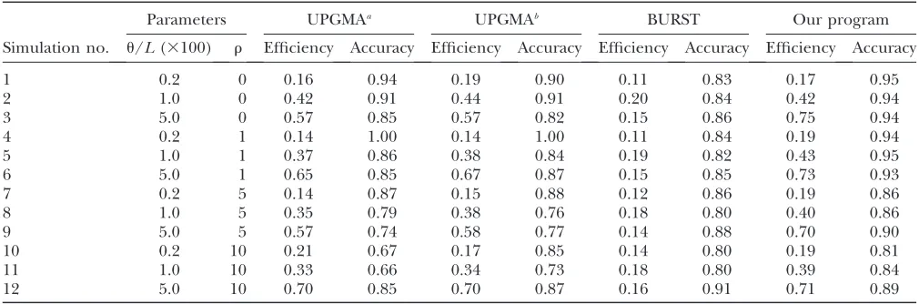
Analysis of simulated data sets shows that despite these potential difficulties our model provides useful results and outperforms existing methods of
Instead of checking convergence for each run we assess the validity of the results by comparison with the true history.
Figure 3 compares our method and eBURST (Feil
et al.2004), an implementation of the BURST algorithm, for one example withu¼0.2 per site, andr¼5 for the entire data set. In this example, it is clearly not going to be possible to infer every branch of the genealogy let alone to accurately estimate each branch length (both shown in Figure 3A) because the 100 isolates have only 27 sequence types between them. We handle the statistical uncertainty by retaining only branches that are supported in a majority-rule consensus tree (Bryant 1997) on the basis of the posterior probability for the genealogy and using the posterior mean for the length of each supported branch (Figure 3B). Our algorithm both correctly captures the overall structure of the tree and correctly infers the sequence types (STs) of most internal nodes (shown in italics on each branch, withx
denoting an ST that is not found in extant strains). One
of the few errors is that the strain with ST 20 is not cor-rectly grouped with STs 7 and 4 on the genealogy in-ferred by our method. An explanation can be found by looking at the sequence types of the ancestral nodes of the real topology: ST 20 was in fact the type of the most recent common ancestor of more than half of the sample. This type disappeared by mutation and recom-bination, but reappeared later once due to recombina-tion. Our program has correctly inferred that the type of the most recent common ancestor (MRCA) of STs 1 and 3 was 20 and therefore clustered the observed isolate of type 20 at that point in the tree, which is the most parsimonious explanation for the observed data but not the correct one in this case.
A UPGMA tree (Figure 3C) correctly captures most of the branch structure of the tree but gets the branching order of the deepest clades wrong (i.e., in the true tree ST 3 is more closely related to ST 2 than to ST 11 while the UPGMA tree indicates the opposite). Another issue is that many branch lengths are exaggerated (e.g., ST 21).
TABLE 2
Comparison of the efficiency and accuracy of UPGMA using site-by-site and gene-by-gene bootstrapping, BURST, and our method on simulated data
Parameters UPGMAa UPGMAb BURST Our program
Simulation no. u/L(3100) r Efficiency Accuracy Efficiency Accuracy Efficiency Accuracy Efficiency Accuracy
1 0.2 0 0.16 0.94 0.19 0.90 0.11 0.83 0.17 0.95
2 1.0 0 0.42 0.91 0.44 0.91 0.20 0.84 0.42 0.94
3 5.0 0 0.57 0.85 0.57 0.82 0.15 0.86 0.75 0.94
4 0.2 1 0.14 1.00 0.14 1.00 0.11 0.84 0.19 0.94
5 1.0 1 0.37 0.86 0.38 0.84 0.19 0.82 0.43 0.95
6 5.0 1 0.65 0.85 0.67 0.87 0.15 0.85 0.73 0.93
7 0.2 5 0.14 0.87 0.15 0.88 0.12 0.86 0.19 0.86
8 1.0 5 0.35 0.79 0.38 0.76 0.18 0.80 0.40 0.86
9 5.0 5 0.57 0.74 0.58 0.77 0.14 0.88 0.70 0.90
10 0.2 10 0.21 0.67 0.17 0.85 0.14 0.80 0.19 0.81
11 1.0 10 0.33 0.66 0.34 0.73 0.18 0.80 0.39 0.84
12 5.0 10 0.70 0.85 0.70 0.87 0.16 0.91 0.71 0.89
aSite-by-site bootstrapping. bGene-by-gene bootstrapping.
TABLE 3
Comparison of the efficiency and accuracy of our method for different sizes of simulated data
73500 bp 143500 bp
Simulation no. u/L(3100) r Efficiency Accuracy u/L(3100) r Efficiency Accuracy
1 0.2 0 0.17 0.95 0.2 0 0.28 0.96
2 1.0 0 0.42 0.94 1.0 0 0.58 0.94
3 5.0 0 0.75 0.94 5.0 0 0.84 0.96
4 0.2 1 0.19 0.94 0.2 2 0.23 0.96
5 1.0 1 0.43 0.95 1.0 2 0.54 0.96
6 5.0 1 0.73 0.93 5.0 2 0.84 0.94
7 0.2 5 0.19 0.86 0.2 10 0.27 0.86
8 1.0 5 0.40 0.86 1.0 10 0.53 0.90
Indeed the correlation coefficient between the time of divergence between pairs of strains and their number of nucleotide differences on which UPGMA is based is 0.91, whereas the times inferred by our method have a correla-tion coefficient of 0.97 with the true values. The UPGMA tree also does not make it explicit which STs constitute monophyletic clusters (e.g., ST 11 does not since it occurs in more than one place in the true tree).
eBURST (Figure 3D) correctly identifies many of the subdivisions at the tips of the tree. However, it fails to identify any of the deep nodes in the tree, for example, failing to indicate that ST 11 and ST 14 are related to each other, and also fails to find close relatives for ST 25 or ST 26. Moreover, although it sometimes assigns an-cestral sequences to particular lineages these assign-ments are not particularly accurate (for example, ST 23 is not ancestral to ST 3). A similar network representa-tion of the consensus genealogy (without estimated branch lengths) obtained using our method is shown in Figure 3E. This representation, which should be partic-ularly useful for large data sets, makes it explicit that some STs (for example, ST 2) probably occur in more than one location in the true genealogy, while others probably form a single cluster (such as ST 17). Indeed in this case, inspection of the true genealogy shows that some ST 2 isolates are more closely related to ST 17 isolates than they are to some of the other ST 2’s.
More formally, two types of error can be identified for the branching pattern. An error of type A happens, for example, for STs 1, 9, and 12, where the clustering of these three STs is correctly identified by our method, but the details of how these three STs relate to each other was not inferred. We call efficiency the ratio of numbers of correctly inferred clusters and clusters pres-ent in the data (this second number being always equal toN1). An error of type B happens, for example, for ST 20, which is not inferred to be a close relative of 4 as it should be, causing the cluster containing STs 4 and 7 to be wrong. We call accuracy the proportion of inferred clusters that are correct. For this example the efficiency of our program is 18% and its accuracy is 90%. Exactly the same method can be used to measure the perfor-mance of BURST (which we reimplemented ourselves for the purpose of comparison). We interpreted BURST output as a genealogy analogous to ours. Specifically we assume that only STs at the tips of each complex and groups of STs that form a single clade radiating from the ancestral ST are predicted to be monophyletic. Ac-cording to these criteria, the efficiency of BURST is 13% and its accuracy is 68%. The alternative assumption that each ST constitutes a monophyletic lineage gives an in-crease in efficiency, but at the expense of a large de-crease in accuracy (data not shown).
We have performed simulations of 10 ARGs similar to the one presented above for a range of parameter com-binations (u, r), which shows that our algorithm pro-vides accurate subdivisions and outperforms existing
methods (Table 2). BURST has consistent accuracy of 80–91% for all parameter combinations we explored but never infers.20% of the nodes correctly, even when there are a large number of mutations on the tree, so that the data are potentially highly informative about relationships between strains.
UPGMA trees can be bootstrapped either site-by-site or gene-by-gene. The latter takes into account the pro-perty that recombination can import an entire gene that may look similar to the sequence of another strain. Gene-by-gene bootstrapping performs more accurately for high recombination rates but both methods gener-ally underperform our program in both accuracy and efficiency. The efficiency of our method is significantly increased for all parameter combinations by doubling the number of loci to 14, showing that additional se-quencing is likely to be effective in providing additional resolution (Table 3).
In general, the performance of our method increases with uand decreases with r. For low values ofu (sim-ulations 1, 4, 7, and 10), the accuracy and efficiency of our program is only slightly better than that of boot-strapped UPGMA trees. However, for higher values ofu (simulations 3, 6, 9, and 12), our program outperforms bootstrapped UPGMA trees both in accuracy and in efficiency by up to 10% (simulations 3 and 9).
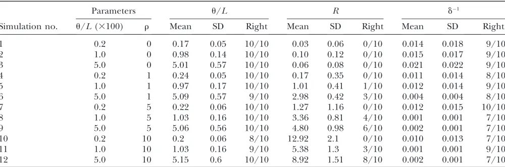
Our model can also be used to estimate model param-eters (Table 4). It provides accurate and approximately unbiased estimates ofuand the size of imported chunks, d. Estimates for the recombination raterare poor when r andu are low (simulations 1–7 and 10) but become better for higher values of these two parameters (sim-ulations 9 and 12).
Application to a Bacillus MLST data set: Finally,
we present a reanalysis of the Bacillus data set described in Priestet al.(2004). We calculated a 95% majority-rule consensus genealogy assuming no recombination (Figure 4A) and estimating recombination parameters and location of imports from the data (Figure 4B), on the basis of 100,000 iterations including 50,000 burn-in iterations, which required6 hr on a desktop com-puter. This consensus was highly replicable between different runs of the algorithm. Figure 4D shows the location of imports for each of the seven MLST loci estimated for a selection of branches as indicated in Figure 4B.
genetic import in thepycAgene in the common ances-tor of the latter three STs (corresponding to event G in Figure 4D) obscured this close relationship. Third, statistical support for some subdivisions, such as many of those within the Kurstaki clade, is overestimated. Indeed, the topmost node in our genealogy, indicating the relationships between Kurstaki, Cereus, and Others, is not resolved, consistent with the general difficulty in inferring deep branches when substantial recombina-tion has taken place.
Our analysis confirms and refines the original con-clusions of Priestet al.(2004), namely that some of the named groupings of Bacillus do not correspond to mono-phyletic groups, so that the taxonomy needs to be rede-fined. Our method provides the most accurate basis to date for redefining this taxonomy. The inferred value of nis high with a 95% credibility region of 0.031–0.042 and some events have even higher values (e.g., event G in Figure 4D introduces substitutions at a rate of 0.06). Such events introduce a higher rate of polymorphism than is available in the Bacillus population studied (2.5–3.0%), which means that they might come from outside Bacillus. These imports have greatly increased average branch lengths, accounting for the size differ-ence between Figure 4A and 4B. Thus, standard meth-ods of inference assuming a coalescent model with within-population recombination would be particularly inappropriate for this data set. The average tract length of recombination chunksdis surprisingly small with a 95% credibility region of 193–435 bp; however, this low value may in part be due to model misspecification and the fact that the gene fragments of the Bacillus MLST scheme are quite short (405 bp on average), making inference of tract size more difficult.
Our method also produces estimates of the relative frequency of recombination and mutation. However, the limited information provided by short sequence
frag-ments and the wide variety of estimates obtained by different methods suggest that these estimates should also be treated with care. Two quite different measures have been used: the ratio of probabilities that an in-dividual nucleotide will be altered through recombina-tion and point mutarecombina-tion,r/m, and the ratio of absolute number of events r/u. ForNeisseria meningitidis, three quite different methods have been used to estimater/m. Our method, using the data set of Jolleyet al.(2005), which ran for 100,000 iterations including 50,000 of burn in, gives 5–8; a population genetic method based on the pattern of linkage disequilibrium within sequence fragments (McVeanet al.2002) gives 6–16; and a method based on the number of nucleotide changes within single-locus variants of robustly assigned clonal found-ers gives 80 (Feil et al. 1999, 2000, 2001). The three published estimates ofr/u are more consistent, each in-cluding 1. These are our estimate (0.7–1.2), the estimate of Jolleyet al. (2005) (0.16–1.8), and that of Fraser
et al.(2005) based on the distribution of allele sharing within a population (1.1). For Bacillus, 95% credibility regions forr/mandr/ubased on our method are 1.3– 2.8 and 0.2–0.5, respectively, showing that recombina-tion is rare compared to the level observed in Neisseria or in many other bacteria.
eBURST finds few clades in this example, reflecting a paucity of single-locus variants, implying that the STs are too distantly related to be clustered by this type of method (Figure 4C). Our method finds many more sub-divisions, which is analogous to the better performance of our method for high values ofuin the simulated data. Specifically, eBURST has correctly grouped STs 25 and 8 together. Looking at the events on branches A and C on our output indicates that the difference between these two types is a single mutation on theglpFgene, making them single-locus variants of each other. However, eBURST does not see that ST 15 is also a close relative
TABLE 4
Parameter estimation on simulated data
Parameters u/L R d1
Simulation no. u/L(3100) r Mean SD Right Mean SD Right Mean SD Right
1 0.2 0 0.17 0.05 10/10 0.03 0.06 0/10 0.014 0.018 9/10
2 1.0 0 0.98 0.14 10/10 0.10 0.12 0/10 0.015 0.017 9/10
3 5.0 0 5.01 0.57 10/10 0.06 0.08 0/10 0.021 0.022 9/10
4 0.2 1 0.24 0.05 10/10 0.17 0.35 0/10 0.011 0.014 8/10
5 1.0 1 0.97 0.17 10/10 1.01 0.41 1/10 0.012 0.014 9/10
6 5.0 1 5.09 0.57 9/10 2.98 0.42 3/10 0.004 0.004 8/10
7 0.2 5 0.22 0.06 10/10 1.27 1.16 0/10 0.012 0.015 10/10
8 1.0 5 1.03 0.16 10/10 3.36 0.81 4/10 0.001 0.001 7/10
9 5.0 5 5.06 0.56 10/10 4.80 0.98 6/10 0.002 0.001 7/10
10 0.2 10 0.2 0.06 8/10 12.92 2.1 0/10 0.010 0.013 7/10
11 1.0 10 1.03 0.16 9/10 5.38 1.3 3/10 0.001 0.001 9/10
because two mutations, one on glpF and one on tpi, separate it from ST 8. A less stringent definition of clonal complexes would allow these strains to be grouped together but would not help to spot a relationship where several genes have been altered through point muta-tions. Examples of this are branches D, E, and F: many genes have been mutated, but in a pattern consistent with clonal evolution.
DISCUSSION
We have described a general method for using multi-locus sequence data to assess the clonal relationships among a sample of bacteria. As well as defining lineages,
the ancestor, and the recombination and mutation events that have taken place in giving rise to each of its descendants.
Application of our method to simulated data sets shows that as well as providing additional information that existing methods do not, our method provides more accurate subdivisions and appropriate measures of statistical uncertainty. Further, our method is uni-quely able to fully and appropriately utilize information from long stretches of contiguous sequence, up to com-plete genomes. Although our method is slower than non-model-based approaches such as UPGMA trees or the BURST algorithm, the time taken to perform each iteration is a linear function of the product of the number
N of strains and the length L of the sequences. The algorithm should be run for longer asNincreases, but the algorithm remains feasible to apply to scores of bacterial genomes or MLST data from thousands of isolates.
Most problems in bacterial epidemiology and system-atics require accurate information about genealogies, whether on a very short timescale (e.g., in tracking the origin of a particular disease outbreak) or on a longer one (e.g., in identifying lineages that have acquired spe-cific phenotypes), ranging up to species splits. On short timescales, the dominant paradigm has been to identify either isolates with identical STs or ‘‘clonal complexes,’’
i.e., groups of closely related genotypes that share a re-cent common ancestor, on the basis of sharing a partic-ular number of alleles. Over longer timescales, analysis is typically performed using phylogenetic methods, on the basis of a large number of concatenated fragments (Geverset al.2005). Our method allows us to estimate degrees of relatedness at a wide range of different time-scales using a single unified approach. Indeed applica-tion of our method correctly indicates that sharing the same ST can provide quite different information on when the strains last shared a common ancestor, de-pending on the genotypes of the rest of the sample. ST complexes can also differ considerably in their antiquity. Since the method provides indications of uncertainty it also indicates when there is insufficient information to infer clonal relationships in a given data set.
An advantage of model-based approaches overad hoc
methods is that they can be refined to take into account a wide variety of features of the data. For example, instead of the Jukes–Cantor model for mutation used here, it would be possible to incorporate more sophis-ticated models of mutation, such as those discussed in Whelanet al.(2001). Incorporating such a parametric mutational model into our inferential framework would be straightforward. In addition to assuming a simple mutational model, our method does not take into account insertions, deletions, or rearrangements and can handle only fully aligned sequence data. In princi-ple it might be possible to jointly infer alignment and genealogy (Suchardand Redelings2006). The model we use for the prior on the genealogies is a standard
coalescent that assumes a constant population size. This can be generalized to include population subdivisions and growth as described in Wilson et al. (2003). It would also be possible to allow changes in demographic parameters and mutation or recombination rates in different parts of the genealogy (e.g., Drummondet al. 2005, 2006).
The key assumptions of the model concern recombi-nation. The method does not attempt to model the origin of genetic imports and instead assumes that imports introduce a uniform rate of novel substitutions n. As a consequence, the model tends to underestimate the number of recombinations as opposed to mutation events and can infer incorrect subdivisions, particularly if recombination is frequent compared to mutation. There are a number of different ways of addressing these limitations. For example, it should be relatively easy to assign putative origins for inferred imports on the basis of homology with different sequences from within or external to the data set in question and hence to make inferences on patterns of recombination in bacteria, which can be highly nonrandom (Zhu et al. 2001; Didelotet al.2007; Falushet al.2006).
It might also be possible to incorporate some in-formation on origin of imports directly into the model. For example, for each branch in the genealogy, it would be possible to distinguish between substitutions that are novel and those that are already present in another lineage. Those that are present are more likely to have been introduced by recombination and also provide information about the likely origin of the event. An-other interesting refinement would be to make the sub-stitution rate in recombined regions nonconstant. One way to do this would be to have a different value ofnfor each recombined region, but this implies a nonconstant dimensionality of the parameter space, which requires the use of complex inferential methods, for example, reversible-jump MCMC (Green1995) or exact sampling (Fearnhead 2006). Alternatives include having a dif-ferent value ofnfor each branch or having several pos-sible values ofnrepresenting different distances of the import source. Each of these refinements would make the inference a lot slower unless efficient approxima-tions can be found.
In summary, we find that the method that we described here provides accurate estimation of bacterial genealo-gies and specific genetic changes both for simulated data and for real data. The application of our general ap-proach to the large-scale DNA sequence data sets that are becoming available should facilitate a detailed under-standing of patterns of microevolution and phenotypic change (Falushand Bowden2006) in diverse bacterial genera.
We thank Nick Thomson, Julian Parkhill, and the Sanger Institute for giving us permission to use the unpublished genomes of DT2, DT104, and SL1344. Mark Achtman, Niall Cardin, Paul Fearnhead, Edward Feil, Ana Bele´n Ibarz-Pavo´n, Keith Jolley, Martin Maiden, Geoff Nicholls, Noel McCarthy, Gil McVean, Jonathan Pritchard, Matthew Stephens, Jay Taylor, Joe Watkins, Daniel Wilson, and an anonymous reviewer provided useful comments, ideas, and discussion. This work was funded by the Wellcome Trust.
LITERATURE CITED
Bryant, D., 1997 Hunting for trees, building trees and comparing trees: theory and method in phylogenetic analysis. Ph.D. Thesis, Department of Mathematics, University of Canterbury, Christ-church, New Zealand.
Darling, A. C., B. Mau, F. R. Blattnerand N. T. Perna, 2004 Mauve: multiple alignment of conserved genomic sequence with rear-rangements. Genome Res.14:1394–1403.
Didelot, X., M. Achtman, J. Parkhill, N. R. Thomsonand D. Falush, 2007 A bimodal pattern of relatedness between theSalmonella
paratyphi A and typhi genomes: Convergence or divergence by homologous recombination? Genome Res.17:61–68.
Dingle, K. E., F. M. Colles, D. Falushand M. C. Maiden, 2005 Se-quence typing and comparison of population biology of Campylo-bacter coliandCampylobacter jejuni.J. Clin. Microbiol.43:340–347. Donnelly, P., and S. Tavare´, 1995 Coalescents and genealogical
structure under neutrality. Annu. Rev. Genet.29:401–421. Drummond, A., and A. Rambaut, 2003 BEAST v1.0 (http://evolve.
zoo.ox.ac.uk/beast/).
Drummond, A., A. Rambaut, B. Shapiroand O. Pybus, 2005 Bayes-ian coalescent inference of past population dynamics from molecular sequences. Mol. Biol. Evol.22:1185–1192.
Drummond, A. J., S. Y. Ho, M. J. Phillipsand A. Rambaut, 2006 Re-laxed phylogenetics and dating with confidence. PLoS Biol.4:
e88.
Durbin, R., S. Eddy, A. Kroghand G. Mitchison, 1998 Biological
Sequence Analysis: Probabilistic Models of Proteins and Nucleic Acids.
Cambridge University Press, Cambridge/London/New York. Falush, D., and R. Bowden, 2006 Genome-wide association
map-ping in bacteria? Trends Microbiol.14:353–355.
Falush, D., M. Torpdahl, X. Didelot, D. F. Conrad, D. J. Wilson
et al., 2006 Mismatch induced speciation inSalmonella: model and data. Philos. Trans. R. Soc. B361:2045–2053.
Fearnhead, P., 2006 Exact and efficient Bayesian inference for mul-tiple changepoint problems. Stat. Comput.16:203–213. Feil, E., M. Maiden, M. Achtmanand B. Spratt, 1999 The relative
contributions of recombination and mutation to the divergence of clones ofNeisseria meningitidis.Mol. Biol. Evol.16:1496–1502. Feil, E. J., J. M. Smith, M. C. Enrightand B. G. Spratt, 2000 Esti-mating recombinational parameters inStreptococcus pneumoniae
from multilocus sequence typing data. Genetics154:1439–1450. Feil, E. J., E. C. Holmes, M. C. Enright, D. E. Bessen, N. P. J. Day
et al., 2001 Recombination within natural populations of path-ogenic bacteria: short-term empirical estimates and long-term phylogenetic consequences. Proc. Natl. Acad. Sci. USA98:182– 187.
Feil, E. J., B. C. Li, D. M. Aanensen, W. P. Hanageand B. G. Spratt, 2004 eBURST: inferring patterns of evolutionary descent among clusters of related bacterial genotypes from multilocus sequence typing data. J. Bacteriol.186:1518–1530.
Felsenstein, J., 1989 PHYLIP—phylogeny inference package (ver-sion 3.2). Cladistics5:164–166.
Fraser, C., W. P. Hanageand B. G. Spratt, 2005 Neutral micro-epidemic evolution of bacterial pathogens. Proc. Natl. Acad. Sci. USA102:1968–1973.
Gansner, E. R., and S. C. North, 2000 An open graph visualization system and its applications to software engineering. Softw. Pract. Exper.30:1203–1233.
Gelman, A., and D. B. Rubin, 1992 Inference from iterative simula-tion using multiple sequences. Stat. Sci.7:457–511.
Gevers, D., F. M. Cohan, J. G. Lawrence, B. G. Spratt, T. Coenye
et al., 2005 Re-evaluating prokaryotic species. Nat. Rev. Micro-biol.3:733–739.
Gilks, W. R., S. Richardsonand D. J. Spiegelhalter, 1998 Markov
Chain Monte Carlo in Practice.Chapman & Hall, London/New York. Green, P. J., 1995 Reversible jump Markov chain Monte Carlo compu-tation and Bayesian model determination. Biometrika82:711–732. Griffiths, R., and P. Marjoram, 1996 Ancestral inference from samples of DNA sequences with recombination. J. Comput. Biol.3:479–502. Hudson, R. R., 1983 Properties of a neutral allele model with
intra-genic recombination. Theor. Popul. Biol.23:183–201. Jolley, K. A., E. J. Feil, M.-S. Chanand M. C. J. Maiden, 2001
Se-quence type analysis and recombinational tests (START). Bio-informatics17:1230–1231.
Jolley, K. A., D. J. Wilson, P. Kriz, G. Mcveanand M. C. J. Maiden, 2005 The influence of mutation, recombination, population history, and selection on patterns of genetic diversity inNeisseria meningitidis.Mol. Biol. Evol.22:562–569.
Jukes, T. H., and C. R. Cantor, 1969 Evolution of protein mole-cules, pp. 21–132 in Mammalian Protein Metabolism, edited by H. N. Munro. Academic Press, New York.
Kingman, J. F. C., 1982 The coalescent. Stoch. Proc. Appl.13:235– 248.
Kumar, S., K. Tamura, I. B. Jakobsenand M. Nei, 2001 MEGA2: molecular evolutionary genetics analysis software. Bioinformat-ics17:1244–1245.
Lawrence, J., and H. Hendrickson, 2003 Lateral gene transfer: When will adolescence end? Mol. Microbiol.50:739–749. Maiden, M. C. J., J. A. Bygraves, E. Feil, G. Morelli, J. E. Russell
et al., 1998 Multilocus sequence typing: a portable approach to the identification of clones within populations of pathogenic mi-croorganisms. Proc. Natl. Acad. Sci. USA95:3140–3145. Maynard Smith, J., N. Smith, M. O’Rourke and B. Spratt,
1993 How clonal are bacteria? Proc. Natl. Acad. Sci. USA90:
4384–4388.
McClelland, M., K. E. Sanderson, J. Spieth, S. W. Clifton, P. Latreilleet al., 2001 Complete genome sequence of
Salmo-nella entericaserovar Typhimurium LT2. Nature413:852–856. McVean, G. A., and N. J. Cardin, 2005 Approximating the
coales-cent with recombination. Philos. Trans. R. Soc. Lond. B Biol. Sci.360:1387–1393.
McVean, G., P. Awadallaand P. Fearnhead, 2002 A coalescent-based method for detecting and estimating recombination from gene sequences. Genetics160:1231–1241.
Milkman, R., and M. M. Bridges, 1990 Molecular evolution of the
Escherichia coli chromosome. III. Clonal frames. Genetics126:
505–517.
Milkman, R., and I. Crawford, 1983 Clustered third-base substitu-tions among wild strains ofEscherichia coli.Science221:378–380. Ochman, H., J. G. Lawrenceand E. A. Groisman, 2000 Lateral
gene transfer and the nature of bacterial innovation. Nature
405:299–304.
Priest, F. G., M. Barker, L. W. Baillie, E. C. Holmesand M. C. Maiden, 2004 Population structure and evolution of the
Bacil-lus cereusgroup. J. Bacteriol.186:7959–7970.
Pritchard, J., M. Stephensand P. J. Donnelly, 2000 Inference of population structure using multilocus genotype data. Genetics
155:945–959.
Rabiner, L. R., 1989 A tutorial on hidden Markov models and se-lected applications in speech recognition. Proc. IEEE77:257–286. Roijers, F., M. Mandjesand J.van denBerg, 2007 Analysis of con-gestion periods of an M/M/inf-queue. Performance Evaluation (in press).
Schierup, M. H., and J. Hein, 2000 Consequences of recombina-tion on tradirecombina-tional phylogenetic analysis. Genetics156:879–891. Spratt, B., W. Hanage, B. Li, D. Aanensenand E. Feil, 2004 Dis-playing the relatedness among isolates of bacterial species—the eBURST approach. FEMS Microbiol. Lett.241:129–134. Suchard, M. A., and B. D. Redelings, 2006 BAli-Phy: simultaneous
Bayesian inference of alignment and phylogeny. Bioinformatics
22:2047–2048.
Swofford, D., 2002 PAUP*. Phylogenetic Analysis Using Parsimony
(*and Other Methods), Version 4. Sinauer Associates, Sunderland, MA. Whelan, S., P. Liand N. Goldman, 2001 Molecular phylogenetics: state-of-the art methods for looking into the past. Trends Genet.
17:262–272.
Wilson, I. J., M. E. Wealeand D. J. Balding, 2003 Inferences from DNA data: population histories, evolutionary processes and fo-rensic match probabilities. J. R. Stat. Soc. Ser. A166:155–188. Zhu, P., A.van derEnde, D. Falush, N. Brieske, G. Morelliet al.,
2001 Fit genotypes and escape variants of subgroup IIINeisseria
meningitidis during three pandemics of epidemic meningitis. Proc. Natl. Acad. Sci. USA98:15056–15061.
Communicating editor: M. K. Uyenoyama
APPENDIX A: MARKOVIAN STRUCTURE OF THE RECOMBINED AND UNRECOMBINED REGIONS
Under our model, recombination may happen several times on a branch of the tree and affect the same portion of the genome repetitively. However, because recombination erases previous polymorphism accumulated through recombination and mutation for that branch, it is impossible to tell how many successive recombination events took place. We therefore describe each site of each branch as having two states: imported or unimported. The lengths of imported and nonimported regions follow complex distributions that are, respectively, those of busy and idle periods of anM/M/‘queue with arrival rateRlu/2 and mean service requirementdas studied by Roijerset al.(2007).
To facilitate statistical inference, we approximate the relationship of these two states for a branch of lengthlto make it Markovian with transition matrix from one nucleotide to the next equal to
to to
unimported imported from unimported
from imported
1bðlÞ bðlÞ
aðlÞ 1aðlÞ
: ðA1Þ
Wherea(l)1andb(l)1are set to be equal to the means of the busy and idle periods of anM/M/‘queue, respectively,
aðlÞ ¼ Rlu=2
eRlud=21 and bðlÞ ¼Rlu=2: ðA2Þ
Consequently, the average length of an imported region isa(l)1and the average length of an unimported region isb(l)1.
The imported and unimported states are not observed directly for each branch but the level of polymorphism between the genotypes at the top and the bottom of a branch gives us some information on the state. Under our model, the expected polymorphism rates in affected and unaffected regions arenandul/2L, respectively. We can therefore use a hidden Markov model to infer the location of affected and unaffected regions given the genotype at the top and at the bottom of a branch ofT.
APPENDIX B: UPDATE OF THE ANCESTRAL SEQUENCES AND MAPS OF IMPORT
We consider a nonroot noden. Letaandbdenote the children ofnandfdenote its father. Letln,la, andlbdenote the lengths of the branches aboven,a, andb, respectively. We need to update the ancestral sequencecnand map of imports
rnofn, as well as the map of importsraandrbof the two children ofngiven the rest of the parameters and the data. These depend only onln,la, andlband the ancestral sequencesca,cb, andcfofa,b, andf, so that we need to sample from
Pðcn;rn;ra;rbjln;la;lb;cf;ca;cb;MÞ. To do so, we first sample fromPðrn;ra;rbjln;la;lb;cf;ca;cb;MÞand then sample from
Pðcnjln;la;lb;rn;ra;rb;cf;ca;cb;MÞ.
To sample fromPðrn;ra;rbjln;la;lb;cf;ca;cb;MÞ, we consider the HMM (Durbinet al.1998; Rabiner1989), where at each location the hidden states are the values ofrn,ra, andrband the observed messages are the values ofcf,ca, andcb. This HMM has eight different possible hidden states becausern,ra, andrbtake values in {0, 1} (0 for a nonimported region and 1 for an imported region) and five messages (enumerated in the emission matrix section below). Samples fromPðrn;ra;rbjln;la;lb;cf;ca;cb;MÞare obtained using the forward–backward algorithm, with the transition and emission matrices detailed below. The second step, sampling from Pðcnjln;la;lb;rn;ra;rb;cf;ca;cb;MÞ, is straight-forward: we calculate for each position the probabilities ofcnto be A, C, G, and T givenln,la,lb,rn,ra,rb,cf,ca, andcb at that position and choose one of the four possibilities with their respective probabilities.
Transition matrix:Letpidenote the hidden state at siteiandxidenote the message at sitei. The transition matrix
Emission matrix:The emission matrixEis defined byes,m¼P(xi¼mjpi¼s). Forj2{n,a,b} letmj¼ulj/(2L) ifrjis in a nonimported region andnotherwise. Assuming that there are no repeat mutations on each branch, the emission probabilities inEare equal to (1mn)(1ma)(1mb)1mnmamb/9 for message 1 (cf,ca, andcbare equal), (1ma)(1 mb)mn1mamb(1mn)/312mnmamb/9 for message 2 (cfis different fromcaandcb), (1mn)(1mb)ma1mbmn(1ma)/ 31 2mnmamb/9 for message 3 (cais different fromcfandcb), (1 mn)(1ma)mb1mamn(1mb)/312mnmamb/9 for message 4 (cbis different fromcfandca), and 2(1mn)mamb/312(1ma)mnmb/312(1mb)mnma/312mnmamb/9 for message 5 (cf,ca, andcbare all different).
Forward–backward algorithm:We can use the transition and emission matricesTandEabove to calculate the matrix
F, wherefs,i¼P(x1,. . .,xi,pi¼s). This is done by using the recursion equation
fs;i11¼es;xi11
X
k
fk;itk;s: ðB1Þ
We can then drawpLfromP(pL¼s)¼fs,Land eachpiiteratively for allifromL1 down to 1, using
Pðpi¼sjpi11;xÞ ¼fs;its;pi11: ðB2Þ
The complexity of this algorithm isO(M2L), whereLis the length of the alignment andMthe number of hidden states (eight here). This is acceptable even for full bacterial genomes where the length of an alignment is a few million base pairs, but as this procedure will be called repetitively in the Monte Carlo Markov chain for each internal node of the phylogeny, a considerable proportion of the time will be spent in it and it is therefore interesting to optimize it as much as possible.
Optimization:One way in which this algorithm can be made much faster is to calculate only the values offs,ifor a subset of the sites that we call the ‘‘reference sites.’’ We used the polymorphic sites, the sites at the beginning or end of blocks, and additional sites at intervals of 50 bp. Ifp(i) denotes theith reference site then Equation B1 becomes
fl;pði11Þ¼el;xpði11Þ X
k
fk;pðiÞqðk;l;pði11Þ pðiÞÞ; ðB3Þ
where
qðk;l;pði11Þ pðiÞÞ ¼Pðppði11ÞjppðiÞ;ðxpðiÞ11;xpðiÞ12;. . .;xpði11Þ1Þ ¼1Þ: ðB4Þ
The values ofQcan be calculated recursively, using
qðk;l;1Þ ¼tk;l and qðk;l;d11Þ ¼ X
m
qðk;m;dÞtm;lem;1: ðB5Þ
Note that as the values ofQdo not depend onp(i) andp(i11) but only on their differenced,Qcan be calculated once and for all before applying the forward–backward algorithm for alld¼[1,. . ., maxi2[1,. . .,L1](p(i11)p(i))].
In the backward step, we use the following equation instead of (B2):
ðppðiÞjppði11Þ;xÞ ¼fk;pðiÞqðppðiÞ;ppði11Þ;pði11Þ pðiÞÞ: ðB6Þ
This determines the hidden states at all reference sites. To finish, we determine the hidden states between two reference sites by assuming that there is no change of state when two consecutive polymorphic sites have the same state and assuming that there is only one transition point when they are different. For a transition between statesxandyat distancedfrom each other, the probability that the transition is at a distanceifrom the polymorphic site of statexfor alli2[0,. . .,d] is given by
PðiÞ}ex;1iey;1di1tx;xity;ydi1tx;y: ðB7Þ
It is possible to verify that this approximation has only a minor effect on the behavior of the program by calculating the acceptance ratio of the move as if it was a Metropolis–Hastings move;i.e., the ratio
a¼PðC9;R9j A;T;MÞ PðC;R j A;T;MÞ
QðC;R j C9;R9;A;T;MÞ
QðC9;R9j C;R;A;T;MÞ: ðB8Þ
APPENDIX C: UPDATE OF THE PARAMETER MODELSMAND THE AGES OF THE GENEALOGY
LetMdenote the set of parameters of our model,i.e.,M ¼ fu;R;d;ng. Depending on how much prior information we have on each of these parameters we might want to estimate them or not in the MCMC.
nis the only one that can be updated using a Gibbs step: as the likelihoodPðA;T;C;R j MÞis a binomial function of n, using a conjugate Beta prior fornleads to a Beta-distributed posterior. Here we used a Beta(1, 1) prior forn,i.e., a uniform prior on [0, 1]. A non-Beta prior distribution can also be assumed if we use a Metropolis–Hastings move as described below.
ForR,d1, anduwe have to use a Metropolis–Hastings update. A natural uninformative prior is a uniform prior for the log of each parameter. To make it proper, we consider only values of each parameter between 1010and 1.
We propose to update the value of log(u) by addingsto it withsdrawn uniformly from [0.05; 0.05]. If the proposed value is,1010or.1, the move is rejected. This move is symmetric and its acceptance probability is simply equal to the minimum of one and the ratio of posterior probabilitiesPðT;M;R;C j AÞcalculated using Equation 5.
The ages ofT are updated using Metropolis–Hastings updates. For each internal nodenof the treeT, its age is updated by adding to it a random draw from Unif([0.05, 0.05]). If the new age is,0, less than the age of one of the children ofn, or more than the age of the father ofn, then the move is rejected. The proposal distribution is therefore symmetric and the move is accepted with a probability equal to the minimum of one and the ratio of the likelihood with the new age over the likelihood before the update.
APPENDIX D: DEALING WITH MISSING DATA
There can be several reasons why an alignment contains gaps. First, deletions and insertions in one sequence create indels that correspond to small gaps in the alignment. Second, when aligning genomes against each other, if one sequence is incomplete then gaps may appear in the alignment depending on which alignment method is used. Finally, sequences sometimes contain uncertainty about some of the nucleotides.
Here we treat gaps in the input alignment as missing data. Each missing nucleotide of each sequence in A is therefore considered to be a parameter over which we need to mix as well as for any other parameter. LetGdenote the set of these missing nucleotides. We use a Gibbs step to updateGgivenAand the current values of all the other parameters. Our prior for each missing nucleotide is uniform over the four possible nucleotides.
Clearly, the value of each missing nucleotidegin sequenceadepends only on the valuexat that position in the ancestral sequence of the father ofainT, the valuerof the locations of recombinations on the branch abovea, and the lengthlof the branch abovea: