R E S E A R C H
Open Access
Global dynamics of two systems of
exponential difference equations by
Lyapunov function
Abdul Qadeer Khan
**Correspondence:
[email protected] Department of Mathematics, University of Azad Jammu and Kashmir, Muzaffarabad, Pakistan
Abstract
In this paper, we study the boundedness character and persistence, existence and uniqueness of the positive equilibrium, local and global behavior, and rate of
convergence of positive solutions of two systems of exponential difference equations. Furthermore, by constructing a discrete Lyapunov function, we obtain the global asymptotic stability of the unique positive equilibrium point. Some numerical examples are given to verify our theoretical results.
MSC: 39A10; 40A05
Keywords: difference equations; boundedness; persistence; asymptotic behavior; Lyapunov function; rate of convergence
1 Introduction and preliminaries
Since difference equations and systems of difference equations containing exponential terms have many potential applications in biology, there are many papers dealing with such equations. See, for example the following.
El-Metwallyet al.[] have investigated the boundedness character, asymptotic behavior, periodicity nature of the positive solutions, and stability of the equilibrium point of the following population model:
xn+=α+βxn–e–xn,
where the parametersα,β are positive numbers and the initial conditions are arbitrary non-negative real numbers.
Ozturket al.[] have investigated the boundedness, asymptotic behavior, periodicity, and stability of the positive solutions of the following difference equation:
yn+=
α+βe–yn
γ +yn– ,
where the parametersα,β,γ are positive numbers and the initial conditions are arbitrary non-negative numbers.
Bozkurt [] has investigated the local and global behavior of positive solutions of the following difference equation:
yn+=
αe–yn+βe–yn– γ +αyn+βyn–
,
where the parametersα,β,γ, and the initial conditions are arbitrary positive numbers. Papaschinopouloset al.[] have investigated the boundedness, persistence, and asymp-totic behavior of positive solutions of the following two directional interactive and invasive species models:
xn+=a+bxn–e–yn, yn+=c+dyn–e–xn,
where the parametersa,b,c,dand the initial conditions are arbitrary positive numbers. Papaschinopouloset al.[] have investigated the asymptotic behavior of the solutions of the following three systems of difference equations of exponential form:
xn+=
α+βe–yn
γ+yn–
, yn+=
δ+e–yn
ζ+xn– ,
xn+=
α+βe–yn
γ +xn–
, yn+=
δ+e–xn
ζ+yn– ,
xn+=
α+βe–xn
γ +yn–
, yn+=
δ+e–yn
ζ+xn– ,
where the parametersα,β,γ,δ,,δare positive numbers and the initial conditions are arbitrary non-negative numbers.
Papaschinopoulos and Schinas [] have investigated the asymptotic behavior of the pos-itive solutions of the systems of the two difference equations:
xn+=a+byn–e–yn, yn+=c+dxn–e–xn,
xn+=a+byn–e–xn, yn+=c+dxn–e–yn,
where the parametersa,b,c,d, and the initial conditions are arbitrary positive numbers. Recently, Khan and Qureshi [] have investigated the qualitative behavior of the follow-ing exponential type system of rational difference equations:
xn+=
αe–yn+βe–yn– γ+αxn+βxn–
, yn+=
αe–xn+βe–xn– γ+αyn+βyn–
, n= , , . . . ,
whereα,β,γ,α,β,γ, and the initial conditionsx,x–,y,y–are positive real numbers. Motivated by the above studies, our aim in this paper is to investigate the qualitative be-havior of positive solutions of the following two systems of exponential rational difference equations:
xn+=
αe–yn+βe–yn– γ+αyn+βyn–
, yn+=
αe–xn+βe–xn– γ+αxn+βxn–
and
xn+=
αe–xn+βe–xn– γ+αyn+βyn–
, yn+=
αe–yn+βe–yn– γ+αxn+βxn–
, n= , , . . . , ()
where the parametersα,β,γ,α,β,γ, and the initial conditions are positive real num-bers.
More precisely, we investigate the boundedness character, persistence, existence and uniqueness of positive steady state, local asymptotic stability and global behavior of the unique positive equilibrium point, and rate of convergence of positive solutions of systems () and () which converge to its unique positive equilibrium point. For basic theory and applications of difference equations we refer the reader [–] and references therein.
Let us consider the four-dimensional discrete dynamical system of the form
xn+=f(xn,xn–,yn,yn–), yn+=g(xn,xn–,yn,yn–), n= , , . . . , ()
where f :I×J→I andg:I×J→J are continuously differentiable functions and
I,J are some intervals of real numbers. Furthermore, a solution{(xn,yn)}∞n=–of system () is uniquely determined by the initial conditions (xi,yi)∈I×Jfori∈ {–, }. Along
with system () we consider the corresponding vector mapF= (f,xn,g,yn). An equilibrium
point of () is a point (x¯,y¯) that satisfies
¯
x=f(x¯,x¯,y¯,y¯), y¯=g(x¯,x¯,y¯,y¯).
The point (x¯,y¯) is also called a fixed point of the vector mapF.
Definition Let (x¯,y¯) be an equilibrium point of system ().
(i) An equilibrium point(x¯,y¯)is said to be stable if, for everyε> , there existsδ>
such that for every initial condition(xi,yi),i∈ {–, },
i=–(xi,yi) – (x¯,y¯)<δ implies(xn,yn) – (x¯,y¯)<εfor alln> , where · is the usual Euclidean norm inR.
(ii) An equilibrium point(x¯,¯y)is said to be unstable if it is not stable.
(iii) An equilibrium point(x¯,¯y)is said to be asymptotically stable if there existsη>
such thati=–(xi,yi) – (x¯,y¯)<ηand(xn,yn)→(x¯,y¯)asn→ ∞.
(iv) An equilibrium point(x¯,¯y)is called a global attractor if(xn,yn)→(x¯,y¯)asn→ ∞. (v) An equilibrium point(x¯,¯y)is called an asymptotic global attractor if it is a global
attractor and stable.
Definition Let (x¯,y¯) be an equilibrium point of the map
F= (f,xn,g,yn),
wheref andgare continuously differentiable functions at (x¯,y¯). The linearized system of () about the equilibrium point (x¯,y¯) is
where
Xn=
⎛ ⎜ ⎜ ⎜ ⎝
xn
xn–
yn
yn–
⎞ ⎟ ⎟ ⎟ ⎠
andFJ is the Jacobian matrix of system () about the equilibrium point (x¯,y¯).
Lemma [] Consider the system Xn+=F(Xn),n= , , . . . ,whereX is a fixed point of F¯ .
If all eigenvalues of the Jacobian matrix JFaboutX lie inside the open unit disk¯ |λ|< ,then ¯
X is locally asymptotically stable.If any of the eigenvalue has a modulus greater than one,
thenX is unstable¯ .
The following result gives the rate of convergence of solutions of a system of difference equations:
Xn+= A+B(n)
Xn, ()
whereXnis anm-dimensional vector,A∈Cm×mis a constant matrix, andB:Z+→Cm×m
is a matrix function satisfying
B(n)→ ()
asn→ ∞, where · denotes any matrix norm which is associated with the vector norm
(x,y)=x+y.
Proposition (Perron’s theorem) [] Suppose that condition()holds.If Xnis a solution
of(),then either Xn= for all large n or
ρ= lim
n→∞ Xn
/n
or
ρ= lim
n→∞ Xn+
Xn
exists and is equal to the modulus of one of the eigenvalues of matrix A.
2 On the systemxn+1= αe
–yn+βe–yn–1 γ+αyn+βyn–1,yn+1=
α1e–xn+β1e–xn–1 γ1+α1xn+β1xn–1
In this section, we shall investigate the asymptotic behavior of system (). Let (x¯,¯y) be the equilibrium point of system () then
¯
x= (α+β)e –¯y
γ+ (α+β)y¯, y¯=
(α+β)e–x¯ γ+ (α+β)x¯
.
To construct the corresponding linearized form of system (), we consider the following transformation:
where
f = αe
–yn+βe–yn–
γ +αyn+βyn–
, f=xn, g=
αe–xn+βe–xn– γ+αxn+βxn–
, g=yn.
The Jacobian matrix about the fixed point (x¯,y¯) under the transformation () is given by
FJ(x¯,y¯) =
⎛ ⎜ ⎜ ⎜ ⎜ ⎝
–γα(+(α+β)e–¯y+x¯)y¯ –γβ(+(α+β)e–¯y+x¯)¯y
– α(e–¯x+¯y) γ+(α+β)x¯ –
β(e–¯x+¯y)
γ+(α+β)x¯
⎞ ⎟ ⎟ ⎟ ⎟ ⎠.
2.1 Boundedness and persistence
The following theorem shows that every positive solution {(xn,yn)} of system () is
bounded and persists.
Theorem Every positive solution{(xn,yn)}of system()is bounded and persists.
Proof Let{(xn,yn)}be an arbitrary solution of (). From (), we have
xn≤
α+β
γ =U, yn≤
α+β γ
=U, n= , , , . . . . ()
In addition from () and (), we have
xn≥
(α+β)e– α+β
γ
γ+ (α+β)α+β γ
=L, yn≥
(α+β)e–
α+β γ
γ+ (α+β)α+βγ
=L, n= , , . . . . ()
Hence, from () and (), we get
L≤xn≤U, L≤yn≤U, n= , , . . . .
So the proof is complete.
2.2 Existence of invariant set for solutions
Theorem Let{(xn,yn)}be a positive solution of system().Then[L,U]×[L,U]is an
invariant set for system().
Proof For any positive solution{(xn,yn)} of system () with initial conditions x,x–∈ [L,U], andy,y–∈[L,U], we have
x=
αe–y+βe–y– γ+αy+βy–≤
α+β γ
and
x=
αe–y+βe–y– γ+αy+βy–≥
(α+β)e– α+β
γ
γ + (α+β)α+β γ
Moreover,
y=
αe–x+βe–x– γ+αx+βx–
≤α+β γ
and
y=
αe–x+βe–x– γ+αx+βx–≥
(α+β)e–
α+β γ
γ+ (α+β)α+βγ .
Hence,x∈[L,U] andy∈[L,U]. Similarly, one can show that ifxk∈[L,U] and
yk∈[L,U], thenxk+∈[L,U] andyk+∈[L,U].
2.3 Existence and uniqueness of the positive equilibrium and local stability
Theorem Suppose that
η< γ γ+ (α+β)L
+ (α+β)(α+β)e–L
γ+ (α+β)L
, ()
where
η= (α+β)(α+β)e–
(α+β)e–L
γ+(α+β)L–L (γ+α+β) γ+ (α+β)U + (α+β)(α+β)e–L γ+ ( +U)(α+β)
.
Then system()has a unique positive equilibrium point(x¯,y¯)in[L,U]×[L,U].
Proof Consider the following system of equations:
x= (α+β)e –y
γ+ (α+β)y, y=
(α+β)e–x γ+ (α+β)x
.
Let F(x) = γ(α+β)+(α+β)e–ff((xx)) –x, where f(x) = (α+β)e–x
γ+(α+β)x andx∈[L,U]. Then it follows that F(L) = (α+β)e
–f(L)
γ+(α+β)f(L)–L. Now,F(L) > if and only if
(α+β)e–
(α+β)e–L
γ+(α+β)L >L
γ +(α+β)(α+β)e –L
γ+ (α+β)L
.
Furthermore, we haveF(U) =γ+(α+β)(α+β)e–ff((UU)
)–Uwheref(U) =
(α+β)e–U
γ+(α+β)U. It is easy to see thatF(U) < if and only if
(α+β)e–
(α+β)e–U
γ+(α+β)U <U
γ+(α+β)(α+β)e –U
γ+ (α+β)U
.
Hence,F(x) has at least one positive solution in [L,U]. Furthermore, assume that condi-tion () is satisfied, then one has
dF(x)
dx < – +
η
(γ(γ+ (α+β)L) + (α+β)(α+β)e–L)(γ+ (α+β)L) < .
Theorem Assume that
(α+β)(α+β) e–L+U e–L+U
< γ + (α+β)L γ+ (α+β)L
.
Then the unique positive equilibrium point(x¯,¯y)in[L,U]×[L,U]of system()is locally asymptotically stable.
Proof The characteristic polynomial of the Jacobian matrixFJ(x¯,y¯) about the equilibrium
point (x¯,y¯) is given by
P(λ) =λ– αα(e
–¯y+x¯)(e–x¯+¯y)
(γ+ (α+β)y¯)(γ+ (α+β)x¯)
λ– (αβ+βα)(e
–y¯+x¯)(e–¯x+y¯)
(γ + (α+β)y¯)(γ+ (α+β)x¯) λ
– ββ(e
–y¯+x¯)(e–¯x+y¯)
(γ + (α+β)y¯)(γ+ (α+β)x¯) .
Let(λ) =λand
(λ) = αα(e
–¯y+x¯)(e–x¯+y¯)
(γ + (α+β)¯y)(γ+ (α+β)x¯)
λ+ (αβ+βα)(e
–¯y+x¯)(e–x¯+y¯)
(γ+ (α+β)y¯)(γ+ (α+β)x¯) λ
+ ββ(e
–¯y+x¯)(e–x¯+y¯)
(γ+ (α+β)y¯)(γ+ (α+β)x¯) .
Assume that (α+β)(α+β)(e–L+U)(e–L+U) < (γ+ (α+β)L)(γ+ (α+β)L). Then one has
(λ)≤ αα(e
–¯y+x¯)(e–x¯+y¯)
(γ + (α+β)¯y)(γ+ (α+β)x¯)
+ (αβ+βα)(e
–¯y+x¯)(e–x¯+y¯)
(γ+ (α+β)y¯)(γ+ (α+β)x¯)
+ ββ(e
–y¯+x¯)(e–x¯+y¯)
(γ+ (α+β)y¯)(γ+ (α+β)x¯)
= (αα+αβ+βα+ββ)
(e–¯y+x¯)(e–x¯+y¯)
(γ+ (α+β)y¯)(γ+ (α+β)x¯)
< (α+β)(α+β)(e
–L+U)(e–L+U)
(γ+ (α+β)L)(γ+ (α+β)L) < .
Then, by Rouche’s theorem,(λ) and(λ) –(λ) have the same number of zeroes in an open unit disk|λ|< . Hence, the unique positive equilibrium point (x¯,y¯) in [L,U]×
[L,U] of system () is locally asymptotically stable.
2.4 Global character
Theorem If
(α+β)e–L<x¯ γ + (α+β)L
and (α+β)e–L<¯yγ+ (α+β)L
, ()
then the unique positive equilibrium point (x¯,y¯)of system()is globally asymptotically stable.
Vn=x¯
The nonnegativity ofVnfollows from the following inequality:
x– –lnx≥, ∀x> .
Assume that () holds true, then it follows that
Vn+–Vn=x¯
for all n ≥ . Thus Vn is a non-increasing non-negative sequence. It follows that
limn→∞Vn ≥ . Hence, we obtain limn→∞(Vn+ – Vn) = . Then it follows that
limn→∞xn+=x¯ andlimn→∞yn+ =y¯. Furthermore,Vn≤Vfor alln≥, which shows that (x¯,y¯)∈[L,U]×[L,U] is uniformly stable. Hence, the unique positive equilibrium point (x¯,y¯)∈[L,U]×[L,U] of system () is globally asymptotically stable.
2.5 Rate of convergence
In this section, we will determine the rate of convergence of a solution that converges to the unique positive equilibrium point of system ().
Let{(xn,yn)}be any solution of system () such thatlimn→∞xn=x¯, andlimn→∞yn=y¯.
To find the error terms, note that
– αx¯(yn–y¯)
So, the limiting system of the error terms can be written as
which is similar to the linearized system of () about the equilibrium point (x¯,y¯). Using Proposition , one has the following result.
Theorem Assume that{(xn,yn)}be a positive solution of system()such thatlimn→∞xn=
of every solution of()satisfies both of the following asymptotic relations:
lim
In this section, we shall investigate the asymptotic behavior of system (). Let (x¯,y¯) be the equilibrium point of system (), then
¯
To construct the corresponding linearized form of system (), we consider the following transformation:
The Jacobian matrix about the fixed point (x¯,y¯) under transformation () is given by
Proof Let{(xn,yn)}be an arbitrary solution of (), then
This proves the statement.
Theorem Let{(xn,yn)}be a positive solution of system().Then[L,U]×[L,U]is an
invariant set for system().
Proof Follows by induction.
3.2 Existence and uniqueness and local stability
The following theorem shows the existence and uniqueness of the positive equilibrium point of system ().
Proof Consider the following system of algebraic equations:
only ife–(e –U
U –αγ+β)< (e–U
U – γ α+β)(U+
γ
α+β). Hence,F(x) has at least one positive solution in [L,U]. Furthermore, assume that condition () is satisfied, then one has
F(x) = (x+ )e
–(x+e–xx–αγ+β)
(e–xx –α+βγ + )
x(e–x x –
γ α+β)
–
≤(U+ )e
–(L+e –L L –
γ α+β)(e–L
L – γ α+β+ )
L (e
–L
L – γ α+β)
– < .
Hence,F(x) = has a unique positive solution in [L,U]. This completes the proof.
Theorem If
(α+β)(α+β) e–L–L+UU
< ( –U–U) γ+ (α+β)L γ+ (α+β)L
, ()
then the unique positive equilibrium point(x¯,y¯)of system()is locally asymptotically sta-ble.
Proof The characteristic equation of the Jacobian matrixFJ(x¯,y¯) about the equilibrium
point (x¯,y¯) is given by
λ–pλ+pλ+pλ+p= ,
wherep=A+C,p=AC–B–AC–D,p=AD–AD+BC–BC,p=BD–BD. Assuming condition () one has
i=
|pi|=
(α+β)e–x¯
γ + (α+β)¯y+
(α+β)e–y¯ γ+ (α+β)x¯
+(αα+αβ+αβ+ββ)e
–x¯–¯y+ (αα
+αβ+αβ+ββ)x¯y¯ (γ + (α+β)¯y)(γ+ (α+β)x¯)
=x¯+y¯+ (α+β)(α+β)(e
–x¯–y¯+x¯y¯)
(γ + (α+β)¯y)(γ+ (α+β)x¯)
<U+U+
(α+β)(α+β)(e–L–L+UU) (γ+ (α+β)L)(γ+ (α+β)L)
< . ()
Therefore, inequality () and Remark .. of reference [] implies that the unique pos-itive equilibrium point (x¯,y¯) of system () is locally asymptotically stable. This completes
the proof.
3.3 Global character
Theorem If
(α+β)e–L<x¯ γ+ (α+β)L
and (α+β)e–L <¯yγ+ (α+β)L
, ()
Proof Using arrangements for the proof of Theorem and assume that () holds true,
system () is globally asymptotically stable.
3.4 Rate of convergence
In this section we will determine the rate of convergence of a solution that converges to the unique positive equilibrium point of system ().
Let{(xn,yn)}be any solution of system () such thatlimn→∞xn=x¯, andlimn→∞yn=y¯.
To find the error terms,
From () and (), we have
So, the limiting system of the error terms can be written as
⎛
which is similar to linearized system of () about the equilibrium point (x¯,¯y). Using Propo-sition , one has the following result.
of every solution of()satisfies both of the following asymptotic relations:
lim
n→∞en
n =λ
,,,FJ(x¯,y¯), lim n→∞
en+
en
=λ,,,FJ(x¯,y¯),
whereλ,,,FJ(x¯,y¯)are the roots of the characteristic polynomial of FJ(x¯,y¯).
4 Examples
In order to verify our theoretical results and to support our theoretical discussions, we consider several interesting numerical examples. These examples represent different types of qualitative behavior of solutions of the systems of nonlinear difference equations () and (). All plots in this section are drawn with Mathematica.
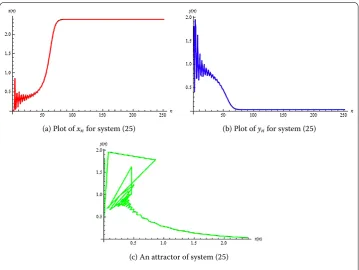
Example Letα= .,β= ,,γ = ,,α= ,,β= ,,γ= ,. Then
system () can be written as
xn+=
.e–yn+ ,e–yn– , + .yn+ ,yn–
, yn+=
,e–xn+ ,e–xn– , + ,xn+ ,xn–
, ()
with initial conditionsx–= .,x= .,y–= .,y= ..
In this case the unique positive equilibrium point of system () is given by (x¯,¯y) = (., .). Moreover, in Figure the plot ofxnis shown in Figure (a), the plot
ofynis shown in Figure (b), and an attractor of system () is shown in Figure (c).
(a) Plot ofxnfor system () (b) Plot ofynfor system ()
(c) An attractor of system ()
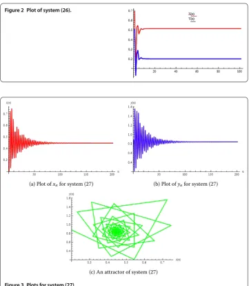
Figure 2 Plot of system (26).
(a) Plot ofxnfor system () (b) Plot ofynfor system ()
(c) An attractor of system ()
Figure 3 Plots for system (27).
Example Letα= ,β= ,γ = ,α= ,β= ,γ= . Then system () can be written as
xn+=
e–yn+ e–yn– + yn+ yn–
, yn+=
e–xn+ e–xn– + xn+ xn–
, n= , , . . . , ()
with initial conditionsx–= .,x= .,y–= .,y= .. The plot of system () is shown in Figure .
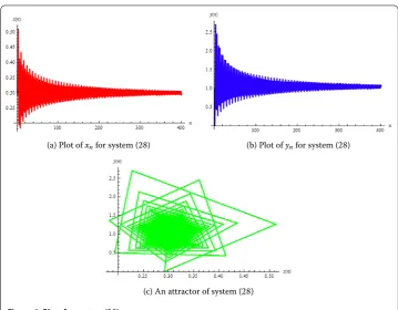
Example Letα= ,β= .,γ = ,α= .,β= .,γ= .. Then system () can be written as
xn+=
e–xn+ .e–xn– + yn+ .yn–
, yn+=
.e–yn+ .e–yn– . + .xn+ .xn–
, ()
(a) Plot ofxnfor system () (b) Plot ofynfor system ()
(c) An attractor of system ()
Figure 4 Plots for system (28).
In this case the unique positive equilibrium point of system () is given by (x¯,¯y) = (., .). Moreover, in Figure the plot ofxnis shown in Figure (a), the
plot ofynis shown in Figure (b), and an attractor of system () is shown in Figure (c).
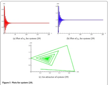
Example Letα= ,β= .,γ = ,α= .,β= .,γ= .. Then system () can be written as
xn+=
e–xn+ .e–xn– + yn+ .yn–
, yn+=
.e–yn+ .e–yn– . + .xn+ .xn–
, ()
with initial conditionsx–= .,x= .,y–= .,y= ..
In this case the unique positive equilibrium point of system () is given by (x¯,¯y) = (., .). Moreover, in Figure the plot ofxnis shown in Figure (a), the plot
ofynis shown in Figure (b), and an attractor of system () is shown in Figure (c).
Example Letα= ,β= .,γ = ,α= ,β= ,γ= .. Then system () can
be written as
xn+=
e–xn+ .e–xn– + yn+ .yn–
, yn+=
e–yn+ e–yn– . + xn+ xn–
, ()
with initial conditionsx–= .,x= .,y–= .,y= ..
In this case the unique positive equilibrium point of system () is given by (x¯,¯y) = (., .). Moreover, in Figure the plot ofxnis shown in Figure (a), the plot
(a) Plot ofxnfor system () (b) Plot ofynfor system ()
(c) An attractor of system ()
Figure 5 Plots for system (29).
Example Letα= ,,β= ,γ = ,,α= .,β= ,γ= .. Then system () can be written as
xn+=
,e–xn+ e–xn– , + ,yn+ yn–
, yn+=
.e–yn+ e–yn– . + .xn+ xn–
, ()
with initial conditionsx–= .,x= .,y–= .,y= ..
In this case the unique positive equilibrium point of system () is unstable. Moreover, in Figure the plot ofxnis shown in Figure (a), the plot ofynis shown in Figure (b), and
a phase portrait of system () is shown in Figure (c).
Example Letα= ,,β= ,γ = ,,α= ,β= ,γ= . Then system () can be written as
xn+=
,e–xn+ e–xn– , + ,yn+ yn–
, yn+=
e–yn+ e–yn– + xn+ xn–
, ()
with initial conditionsx–= .,x= .,y–= .,y= ..
In this case the unique positive equilibrium point of system () is unstable. Moreover, in Figure the plot ofxnis shown in Figure (a), the plot ofynis shown in Figure (b), and
a phase portrait of system () is shown in Figure (c).
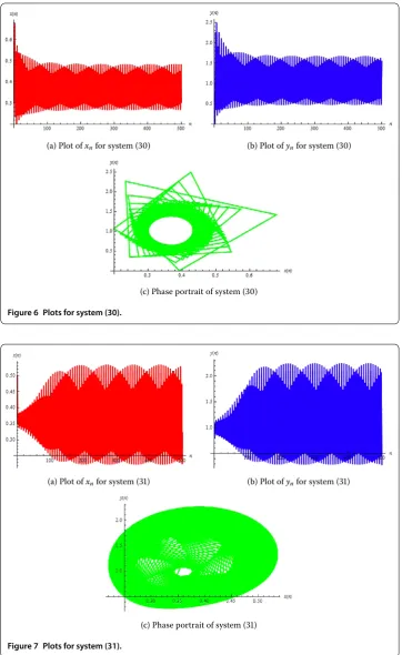
Example Letα= ,,β= ,γ = ,,α= ,β= ,γ= . Then system () can be written as
xn+=
,e–xn+ e–xn– , + ,yn+ yn–
, yn+=
e–yn+ e–yn– + xn+ xn–
, ()
(a) Plot ofxnfor system () (b) Plot ofynfor system ()
(c) Phase portrait of system ()
Figure 6 Plots for system (30).
(a) Plot ofxnfor system () (b) Plot ofynfor system ()
(c) Phase portrait of system ()
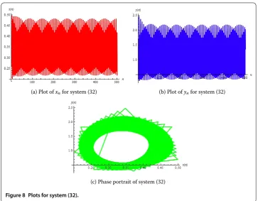
(a) Plot ofxnfor system () (b) Plot ofynfor system ()
(c) Phase portrait of system ()
Figure 8 Plots for system (32).
In this case the unique positive equilibrium point of system () is unstable. Moreover, in Figure the plot ofxnis shown in Figure (a), the plot ofynis shown in Figure (b), and
a phase portrait of system () is shown in Figure (c).
5 Conclusion
This work is related to the qualitative behavior of some systems of exponential rational difference equations. We have investigated the existence and uniqueness of the positive steady state of system () and (). For all positive values of the parameters the boundedness and persistence of positive solutions are proved. Moreover, we have shown that the unique positive equilibrium point of system () and () is locally as well as globally asymptotically stable under certain parametric conditions. The main objective of dynamical systems the-ory is to predict the global behavior of a system based on the knowledge of its present state. An approach to this problem consists of determining the possible global behaviors of the system and determining which parametric conditions lead to these long-term behaviors. By constructing a discrete Lyapunov function, we have obtained the global asymptotic stability of the positive equilibrium of () and (). Finally, some illustrative examples are provided to support our theoretical discussion. First two examples show that the unique positive equilibrium point of system () is stable with different parametric values. Mean-while Examples , , and show that the unique positive equilibrium point of system () is stable whereas the last three examples show that the unique positive equilibrium point of system () is unstable with suitable parametric choices.
Competing interests
The author declares that he has no competing interests.
Author’s contributions
Acknowledgements
The author thanks the main editor and anonymous referees for their valuable comments and suggestions leading to improvement of this paper. This work was supported by the Higher Education Commission of Pakistan.
Received: 25 September 2014 Accepted: 6 November 2014 Published:26 Nov 2014
References
1. El-Metwally, E, Grove, EA, Ladas, G, Levins, R, Radin, M: On the difference equationxn+1=α+βxn–1e–xn. Nonlinear Anal.47, 4623-4634 (2001)
2. Ozturk, I, Bozkurt, F, Ozen, S: On the difference equationyn+1=
α+βe–yn
γ+yn–1 . Appl. Math. Comput.181, 1387-1393 (2006) 3. Bozkurt, F: Stability analysis of a nonlinear difference equation. Int. J. Mod. Nonlinear Theory Appl.2, 1-6 (2013) 4. Papaschinopoulos, G, Radin, MA, Schinas, CJ: On the system of two difference equations of exponential form:
xn+1=a+bxn–1e–yn,yn+1=c+dyn–1e–xn. Math. Comput. Model.54, 2969-2977 (2011)
5. Papaschinopoulos, G, Radin, MA, Schinas, CJ: Study of the asymptotic behavior of the solutions of three systems of difference equations of exponential form. Appl. Math. Comput.218, 5310-5318 (2012)
6. Papaschinopoulos, G, Schinas, CJ: On the dynamics of two exponential type systems of difference equations. Comput. Math. Appl.64(7), 2326-2334 (2012)
7. Khan, AQ, Qureshi, MN: Behavior of an exponential system of difference equations. Discrete Dyn. Nat. Soc.2014, Article ID 607281 (2014). doi:10.1155/2014/607281
8. Din, Q, Qureshi, MN, Khan, AQ: Dynamics of a fourth-order system of rational difference equations. Adv. Differ. Equ.
2012, Article ID 215 (2012)
9. Kulenovi´c, MRS, Ladas, G: Dynamics of Second Order Rational Difference Equations. Chapman & Hall/CRC, London (2002)
10. Elsayed, EM: Solutions of rational difference system of order two. Math. Comput. Model.55, 378-384 (2012) 11. Elsayed, EM: Behavior and expression of the solutions of some rational difference equations. J. Comput. Anal. Appl.
15(1), 73-81 (2013)
12. Elsayed, EM, El-Metwally, H: Stability and solutions for rational recursive sequence of order three. J. Comput. Anal. Appl.17(2), 305-315 (2014)
13. Elsayed, EM, El-Metwally, HA: On the solutions of some nonlinear systems of difference equations. Adv. Differ. Equ.
2013, Article ID 16 (2013)
14. Din, Q, Khan, AQ, Qureshi, MN: Qualitative behavior of a host-pathogen model. Adv. Differ. Equ.2013, Article ID 263 (2013)
15. Khan, AQ, Qureshi, MN, Din, Q: Global dynamics of some systems of higher-order rational difference equations. Adv. Differ. Equ.2013, Article ID 354 (2013)
16. Qureshi, MN, Khan, AQ, Din, Q: Asymptotic behavior of a Nicholson-Bailey model. Adv. Differ. Equ.2014, Article ID 62 (2014)
17. Sedaghat, H: Nonlinear Difference Equations: Theory with Applications to Social Science Models. Kluwer Academic, Dordrecht (2003)
18. Pituk, M: More on Poincaré’s and Perron’s theorems for difference equations. J. Differ. Equ. Appl.8, 201-216 (2002) 19. Enatsu, Y, Nakata, Y, Muroya, Y: Global stability for a class of discrete SIR epidemic models. Math. Biosci. Eng.7(2),
347-361 (2010)
20. Kocic, VL, Ladas, G: Global Behavior of Nonlinear Difference Equations of Higher Order with Applications. Kluwer Academic, Dordrecht (1993)
10.1186/1687-1847-2014-297