Gibbsian method for the self optimization of cellular networks

(1)

R E S E A R C H

Open Access

Gibbsian method for the self-optimization of

cellular networks

Chung Shue Chen

1*

and Franc¸ois Baccelli

2

Abstract

In this study, we propose and analyze a class of distributed algorithms performing the joint optimization of radio resources in heterogeneous cellular networks made of a juxtaposition of macro and small cells. Within this context, it is essential to use algorithms able to simultaneously solve the problems of channel selection, user association and power control. In such networks, the unpredictability of the cell and user patterns also requires distributed

optimization schemes. The proposed method is inspired from statistical physics and based on the Gibbs sampler. It does not require the concavity/convexity, monotonicity or duality properties common to classical optimization problems. Besides, it supports discrete optimization which is especially useful to practical systems. We show that it can be implemented in a fully distributed way and nevertheless achieves system-wide optimality. We use simulation to compare this solution to today’s default operational methods in terms of both throughput and energy consumption. Finally, we address concrete issues for the implementation of this solution and analyze the overhead traﬃc required within the framework of 3GPP and femtocell standards.

1 Introduction

Today’s cellular mobile radio systems strongly rely on highly hierarchical network architectures that allow ser-vice providers to control and share radio resources among base stations and clients in a centralized manner. With the foreseen exponentially increasing number of users and traffic in the 4G and future wireless networks, existing deployment and practice becomes economically unsus-tainable. Network self-organization and self-optimization are among the key targets of future mobile networks so as to relax the heavy demand of human efforts in the network planning and optimization tasks and to reduce the system’s capital and operational expenditure (CAPEX/OPEX) [1-3]. The next-generation mobile net-works (NGMN) are expected to provide a full coverage of broadband wireless service and support fair and efficient radio resource utilization with a high degree of operation autonomy and intelligence.

Due to the emerging high demand of broadband ser-vice and new applications, wireless networking also has to face the challenge of supporting fast increasing data

*Correspondence: [email protected]

1Network Technologies, Alcatel-Lucent Bell Labs, Centre de Villarceaux, 91620 Nozay, France

Full list of author information is available at the end of the article

traffic with the requirement of spectrum and energy uti-lization efficiency [4]. To enhance the network capacity and support pervasive broadband service, reducing cell size is one of the most effective approaches. Deployment of small cell base stations or femtocells has a great poten-tial to improve the spapoten-tial reuse of radio resource and also enhance transmit power efficiency [5]. It is foreseen that the next generation mobile cellular networks will con-sist of heterogeneous macro and small cells with different capabilities including transmit power and coverage range. In such networks due to the unpredictability of the base station and user patterns, network self-organization and self-optimization becomes necessary. Autonomic man-agement and configuration of user association, i.e., assign-ing users to base stations, and radio resource allocation such as transmit power and channel selection would be highly desirable to practical systems [6].

The primary objective of the presented study is to design distributed algorithms performing radio resource alloca-tion and network self-optimizaalloca-tion for today’s macro and small cell (e.g., 3GPP-LTE [2] and femtocell) mixed net-works. In radio resource management, (i) power control, (ii) user association and (iii) channel selection are essen-tial elements. It is known that system-wide radio resource optimization is usually very challenging [7]. A joint opti-mization of user association, channel selection and power

(2)

control is in general non-convex and difficult to solve, even if centralized algorithms are allowed [8]. Notice that in classical networks made of macro cells only, optimizing any of the above three elements independently can effec-tively improve the system performance. However, it may not be true in heterogeneous networks made of a juxta-position of macro and small cells. This would yield extra complexity and difficulties. Besides, future wireless net-works will typically be large, have fairly random topolo-gies, and lack centralized control entities for allocating resources and explicitly coordinating transmissions with global coordination. Instead, these networks will depend on individual nodes to operate autonomously and itera-tively and to share radio resources efficiently. We have to see how individual nodes can perform autonomously and support inter-cell interference management in a dis-tributed way for finding globally optimal configurations.

To begin with, we give two examples to illustrate the problem that may happen when conducting these opti-mizations under macro and small cell networks, in both the downlink and uplink respectively. Consider the down-link scenario in Figure 1 where there are two mobile users uandvunder the macro and small cell base stations (BS) aandbwhich have different maximum transmit powers and coverage ranges. Notice that userucan be covered by the macro cell BSabut it is located near the edge ofas coverage. Meanwhile, it is too close to the small cell BSb and this will have a strong impact on its received signal-to-interference-plus-noise-ratio (SINR). Here, transmit power optimization will not be effective without prior user association and channel selection optimization. One may consider the option in which usersuandvboth asso-ciate with the small cell b. However, this may overload BS b. From the viewpoint of load balancing, it is better to have the two users attached to different cells, e.g., user

User: u Macro cell

BS: a

Small cell BS: b

User: v

Figure 1Since useruis far from its BSa, the received signal at userumay suﬀer strong interference due to the transmission of small cell BSbdestined to userv.

u is attached to BSa. However, useru will then have a low SINR as long as the two transmissions use a same channel. Clearly, one should consider assigning two diﬀer-ent channels for these two transmitter-receiver pairs and hence conduct a joint user association and channel selec-tion optimizaselec-tion with respect to the link characteristics of the possible combinations and their available channels. If the system involves more users and cells, power control should be conducted as well to mitigate interference. This requires a joint optimization of all three elements.

Figure 2 shows a similar problem in the uplink. Con-sider that one first conducts user association optimiza-tion. Since uservis closer to BSbthan to BSa, from the viewpoint of load balancing, the recommended user asso-ciation should be as follows: useruattaches to BSawhile uservattaches to BSb. As useruis far away from its BSa, the transmit power has to be high enough. This will how-ever yield a strong interference to the signal received at BS bwhich is transmitted from userv. Note that in this case, user association optimization, power control or even their joint optimization are not able to solve the problem. However, if one also considers channel allocation and tries to select two different channels for these two transmitter-receiver pairs, a joint optimization will be able to resolve the conflict and enhance overall performance.

Let us now describe what aspects of the problem were considered so far and the novelty of our approach. When each optimization is conducted separately, the proper optimization sequence was studied in [9,10] for the 802.11 WLAN case, based on careful experimental work and sce-nario analysis. Explicit rules were proposed when the cell patterns have a speciﬁc structure (e.g., in the hexagonal base station pattern case). However, for situations where the cell and user patterns are unpredictable as in the small

Small cell BS: b User: v

(3)

cell case, no simple and universal rule is known and a joint optimization is necessary to achieve the best performance. Various separate optimization problems were consid-ered, mainly under the assumptions of centralized coor-dination and global information exchange. For example the transmission powers maximizing system throughput in the multiple interfering link case leads to a non-convex optimization problem which was studied in [11,12]. A power control algorithm that guarantees strict throughput maximization in the general SINR regime is reported in [13]. It is built on multiplicative linear fractional program-ming, which is used for optimization problems expressible as a difference of two convex problems. However, this algorithm requires a centralized control and is only effi-cient for problem instances of small size due to the com-putation complexity. There is a lack of efficient algorithm operating in a distributed manner and ensuring global optimality in the above joint optimization.

Here, we propose and analyze a class of distributed algorithms performing the joint optimization of radio resources in a generalized heterogeneous macro and small cell network. Note that the optimization function does not have qualitative properties such as convexity or mono-tonicity. The proposed solution is inspired from statis-tical physics and based on the Gibbs sampler (see e.g., [14,15]). It is a generalization of the study in [3] which only takes into account power control and user associ-ation and is thus limited to homogeneous mobile cellu-lar networks. The article describes the algorithm, shows that it can be implemented in a fully distributed manner and nevertheless achieves minimal system-wide potential delay, reports on its performance, and analyzes the over-head associated with the information exchange required in the implementation of this solution in today’s 3GPP-LTE and femtocell standards. The rest of the article is organized as follows. Section ‘System model and prob lem formulation’ describes the system model and prob-lem setup. Section ‘Gibbs sampler and self optimization’ presents the proposed solution. Section ‘Simulation and comparison’ compares this solution to today’s default operation in terms of throughput and energy consump-tion. Section ‘Evaluation of overhead traﬃc’ investigates the overhead traﬃc generated by the algorithm. Finally, Section ‘Conclusion’ contains the conclusion.

2 System model and problem formulation

We consider a reuse-1 cellular radio system with a setB of base stations serving a populationU of users. For each useru ∈ U, it is assumed that there is a pair of orthogo-nal channels for the uplink and downlink. We assume that there is no interference between the uplink and downlink and we only consider the downlink. However, the method can be generalized to the uplink as well.

We assume that users can associate with any neighbor-ing base stationb ∈ Bin the network which could be a macro or small cell base station, which is referred to as open access [5]. Today’s default operation attaches each useruto the base station with the highest received power. Note that this is clearly sub-optimal. In general, if one sim-ply associates users with the closest BS or to that with the strongest received signal, it is possible that some BSs have many users while others have only a few. The result-ing overload might lead to a degradation of the network capacity.

Let C be the set of channels (e.g., frequency bands) which are common to all base stations. The base station serving useruis denoted bybu and is restricted to some local set Bu of bases stations (typically Bu is the set of BSs the power of pilot signal of which is received by user uabove some threshold). The channel allocated bybuto user uis denoted cu ∈ C. Here, for simplicity we con-sider that a user only takes one channel. The transmission power used by base stationbutouis denoted byPu.

The SINR at useruis then:

SINR_u= Pul(bu,u,cu)

Nu(cu)+ v∈U,v=u

α(bu,bv,cu,cv)Pvl(bv,u,cv) ,

(1)

whereNu(c)denotes the thermal noise of useruon chan-nelc,l(bu,u,c)is the signal attenuation from BSbutouon channelc, and α(b,b,c,c) represents the orthogonality factor between some user associated with BSbon channel cand some user associated with BSbon channelc.

Note that it makes sense to assume that 0 ≤ α(·) ≤ 1 and that the following symmetry holds: for allb,b,c,c,

α(b,b,c,c)=α(b,b,c,c).

Here are some examples: if adjacent channel interfer-ence is negligible compared to co-channel interferinterfer-ence, then one should takeα(b,b,c,c)=0 forc=c. One may also assume thatα(b,b,c,c)= αandα(b,b,c,c)= βfor b=b, whereαandβare some constants such thatα < β. The simplest case is that whereα=β =1.

Under the additive white Gaussian noise (AWGN) model, the achievable data rate at user u in bit/s/Hz is given by:

ru=Klog(1+SINRu), (2)

where K is a constant depending on the width of the frequency band.

(4)

It aims at minimizing the system-wide potential delay and is explained below.

Instead of maximizing the sum of throughputs, i.e.,

ru, which often leads to very low throughput for some users, we minimize the sum of the inverse of through-put, i.e.,r_u−1, which can be seen as the total delay spent to send an information unit to all the users. Note that minimizingr_u−1penalizes very low throughputs. More explicitly, a bandwidth allocation that provides minimal potential delay fairness is one that minimizes the following cost function:

which is the network’s aggregate transmission delay. It also indicates the long term throughput that a user expects to receive from a fully saturated network.

For mathematical convenience (see below), in this arti-cle, we minimize the cost function

E=

instead of (3). We callE the globalenergy, following the terminology of Gibbs sampling. Note that if one operates in a low SINR regime such that the achievable data rate of a user is proportional to its SINR, e.g.,ru=KSINRu, min-imizing the potential delayCis equivalent to minimizing the global energyE.

Remark 1.E is a surrogate of C. We see that (3) and (4) have quite similar characteristics. The diﬀerence is that

(eruK −1₎−1increases more signiﬁcantly than r−1

u when ru is low. As a result, the overall cost will increase more sub-stantially. So, minimizing E rather than C penalizes low throughputs more signiﬁcantly and favors a higher level of user fairness.

The optimization problem consists in ﬁnding a conﬁg-uration (also referred to as a state) of user association,

channel selection and power allocation which minimizes the above energy function. It is clear that the problem has a high combinatorial complexity and is in general hard to solve for large networks. However the additive struc-ture of the energy can be used to conduct its minimization using a Gibbs sampler. This leverages the decomposition ofEinto a sum of local cost function for each useru(say local energyEu) which can be manipulated in a distributed way in the resource allocation. We explain this setup and optimization in the following section.

3 Gibbs sampler and self optimization

We now describe the distributed algorithm to perform the joint optimization of user association, channel selection and power control. It is based on a Gibbs sampler operat-ing on agraphGof the network which can be deﬁned as follows:

• The set ofnodes inGis the set of users denoted by

u∈U.

• Each nodeu is endowed with a state variablesu

belonging to a ﬁnite setS. The state of a node is a triple describing its user association, its channel and its transmit power; this state denoted by

su= {bu,cu,Pu}. Here, we consider that transmit

power is discretized. We denote the state of the graph bys(su)u∈U.

• Two user nodesu and v are neighbors in this graph if either (i) the powerP0of the pilot signal received

from a possible association base station forv at u is above some threshold, sayθ or (ii) the power received from a possible base station foruis aboveθ atv. We denote the set of neighbors ofubyNu. Notice that v∈Nuif and only ifu∈Nv.

Below, for all subsets V ⊂ U, the cardinality of V is denoted by|V|.

The global energy E = E(s) in (6) derives from a potentialfunctionV(V)[15], that is

E=

V⊆U

V(V), (7)

(5)

A global energy which derives from such a potential function satisfying the conditionV(V) = 0 for|V| ≥ 3 is hence amenable to a distributed optimization using the Gibbs sampler, which is based on the evaluation of the local energy at each node:

Eu=

V⊆Us.t.u∈V

V(V). (8)

Following the above deﬁnition ofV(·), this can be re-written as:

Eu(s)=

Nu(cu)+ v=u,v∈Nu

α(bu,bv,cu,cv)Pvl(bv,u,cv)

Pul(bu,u,cu)

=1/(SINRu)

+

v=u,v∈Nu

α(bv,bu,cv,cu)Pul(bu,v,cu) Pvl(bv,v,cv)

. (9)

The local energy can be written in the following form:

Eu(s)=Au(s)+Bu(s), (10)

where Au(s) and Bu(s) represent the first and second terms of (9), respectively. Notice that the first termAu(s) is equal to 1/SINR_u. It is the “selfish” part of the energy function, which is small whenSINR_uis large. On the other hand, Bu(s) is the “altruistic” part of the energy, which is small when the power of the interference incurred by all the other users because ofuis small compared to the power received from their own base stations.

Remark 2.One can consider thatEuconsists of an indi-vidual cost of u plus another term which corresponds to its impact on the others (v=u).

Remark 3.The above formulation is meant to handle joint power, channel, and user association optimization. However, it can easily be adapted to some special cases, e.g., to the case where the transmit power is a constant.

In the following, we describe more precisely the Gibbs sampler and its properties.

First, we explain what it does. Each BS separately trig-gers a state transition for one of its users picked at ran-dom, sayu, using a local random timer. This transition is selected based on the local energyEu. More precisely, given the state(sv)v=u,v∈Nuof the neighbors ofu, the new statesuis selected in the setSuof potential states for user

u(this set is ﬁnite as power has been quantized to a ﬁnite set) with the probability

πu(su)= e−Eu

(su,(sv)v∈Nu) T

s∈Su

e−Eu

(s,(sv)_v_∈_N_u) T

, su∈Su, (11)

whereT>0 is a parameter called the temperature. We now list the properties of this sampler.

• These local random transitions drive the network to a steady state which is theGibbs distribution associated with the global energy and temperatureT, that is to a state with the following distribution (in steady state):

π_T(s)=c·e−E(s)/T,

withc a normalizing constant. The proof is based on a reversibility argument similar to that of [15].

• This distribution puts more mass on low energy (small cost) conﬁgurations and that whenT→0, the distributionπT(·)converges to a Dirac mass at the

state of minimal cost if it is unique (otherwise to a uniform distribution on the minima).

• This procedure is distributed in that the transition of useru only requires knowledge of the state of its neighbors. We discuss the structure of message exchanges in more detail below.

The exact procedure which users follow to conduct state transitions is summarized in Algorithm 1. Each user sets a timer,tu, which decreases linearly with time. We consider discrete time in step ofδsecond(s) and simply setδ=1. This timer has a duration randomly sampled according to a geometric distribution. Whentuexpires, atransition ofuoccurs by which the state of this user is updated as indicated above.

Greedy variant One may consider to perform the state transition by deterministically choosing the one that max-imizes (11) namely thebest responseinstead of selecting a state according to the Gibbsian probability distribution. It is known that a strategy of best response will drive the system to a local minimum but not necessarily to an opti-mal solution. Some discussions on the price of anarchy of a best response algorithm can be found in [17] and refer-ences therein. The basic idea of the probabilistic approach described above is to keep a possibility to escape from being trapped in a local minimum.

(6)

3.1 Algorithm 1 State transition for the Gibbs sampler.

everyδdo for eachudo

iftu≤0then

for all thesinSudo

Eu(s,(sv,v=u))←Au(s,(sv,v=u)) +Bu(s,(sv,v=u))

du(s,(sv,v=u))← exp(−Eu(s,(sv,v=u))/T); end

samplesu∈Saccording to the probability law π_u(s,(sv,v=u))

du(su)/

s∈Sudu(s,(sv,v=u))

sampletu≥0with distributiongeom(1) else

tu←tu−δ; end

end end

It is known that under conditions which ensure the compactness of the Markov forward operator and the irreducibility of the corresponding chain [18], the Gibbs sampler will converge geometrically fast (forT ﬁxed) to the Gibbs distribution. In Section ‘Simulation and com parison’, we will present simulation results illustrating this convergence.

Annealing variant For a ﬁxed environment (i.e., user population, signal attenuation), if one decreasesT asT = 1/ln(1+t), wheretis time, then the algorithm will drive the network to a state of minimal energy, starting from any state. A concrete proof of this result is similar to that of [15, pp. 311–313]. This proof is based on the notion of weak ergodicity of Markov chains and reversibility argument and is omitted.

3.2 Message exchanges

Two base stations, saybandb, are calledimplicit neigh-borsif there exist two neighboring users u andu such that u can associate to b and u to b, i.e., if b ∈ Bu, b ∈ Bu, and either α(b,b,c,c)P0l(b,u,c) > θ or α(b,b,c,c)P0l(b,u,c) > θfor somec,c. As we shall see, messages have to be exchanged between implicit neighbor base stations only (in addition to those between users and their current association base station).

The necessity for message exchange comes from the need of samplingsuin the algorithm. For this either user u or BS bu (below we assume that the sampling takes place onbu) has to have enough information to determine π_u(s,(sv,v=u)) or equivalentlyEu(s,(sv,v = u))for all s ∈ Su. For this, some measurements and information exchange between neighboring base stations and users are required.

The necessity for message exchange comes from the need of sampling su in the algorithm. For this either useru or its base stationbˆu before the sampling (below we assume that the sampling takes place on bˆu) has to have enough information to determine π_u(s,(sv,v=u)) or equivalentlyEu(s,(sv,v = u))for alls ∈ Su. For this, some measurements and information exchange between neighboring base stations and users are required.

The explicit deﬁnition of Eu in (9), shows that for the evaluation of Au(s), a user u will have to estimate the following data and report them to its base stationbˆu:

1. the receiver noise:Nu(c)on each channelc,

2. the total received interferences:

v=uα(b,bv,c,cv)Pvl(bv,u,c), for eachcand for

eachb∈Bu, and

3. the path-loss or link gain:l(b,u,c), for eachc and for eachb in the setBu.

In order foruorbˆuto evaluateBu(s), for alls∈Su, each userv∈ Nuwill have to estimate the following informa-tion and to report to its own base stainforma-tionbv(which will in turn communicate it to all its implicit neighbors including buon the backhaul network):

1. the power of its received signal:Pvl(bv,v,cv), and

2. the path-loss or link gain:α(bv,b,cv,c)l(b,v,c), for

eachc and for each ofb∈Bu.

Note that the measurement of signal power, interference and path-lossl(b,u,c) for each considered channel from either its own base station or neighboring base stations can be retrieved by the user terminal from for example the measurement of available RSCP (received signal code power) and/or RSSI (received signal strength indication).

By the above information exchange, for each u, base station bû is able to compute Eu for all s ∈ Su and hence to sample the new statesu of useru according to the above algorithm. Notice that inter-cell communica-tion takes place between implicit neighbor base stacommunica-tions only. There is no need to transmit this information via the wireless medium. We assume that this is supported by the backhaul network. The amount of overhead traffic gener-ated by the algorithm can be evalugener-ated. The results on the matter are presented in Section ‘Evaluation of overhead traffic’.

4 Simulation and comparison

A performance investigation of the proposed solution is conducted below. We implement Algorithm 1 and com-pare its performance with today’s 3GPP default operations [19] by discrete event simulations.

(7)

terminals over the covered area. The downlink transmit power is often the maximum allowable power as well for a better user reception and coverage. Note that the pilot sig-nal is broadcasted continuously to allow user equipments (UE) to perform channel measurements and appropriate tuning. In user association, the current practice consists in attaching a user to the BS received with the strongest signal strength (rather than the nearest base station). Note that this could lead to attaching the users to a far macro cell BS which has a higher transmit power than that of a nearer small cell BS. This is in general sub-optimal. In channel allocation, the current practice often follows a heuristic scheme where channels of a BS are assigned to its users simply in a round-robin fashion, i.e., sequentially, and in such a way that the numbers of users on each channels are well balanced and almost equal.

In the simulations, we consider that mobile users are uniformly distributed in a geographic area of 1000 m times 650 m and we adopt the 3GPP-3GPP2 spatial channel model [20]. The distance dependent path-loss is given by:

l(dB)(d)= −30.18−26 log₁₀(d)−X_σ(dB), (12)

wheredis the transmitter-receiver distance andXσrefers to log-normal shadowing with zero mean and standard deviation 4 dB. With operating temperature 290 K and bandwidth 1 MHz, the thermal noise Nu is equal to 4.0039×10−15W, for allu.

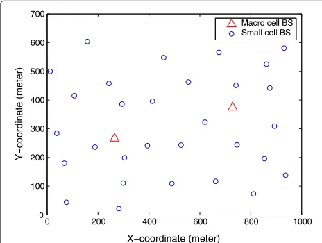
Here we consider that there are two macro cell base stations with ﬁxed locations as shown in Figure 3 and a number of small cell base stations which are randomly located in the geographical area. The maximum transmit power of macro and small cell base stations are 40 and 1 W, respectively. We assume thatPδ=0.1 W. In the sim-ulation, we consider a simple system whereα = 1 and each user only takes one channel.

0 200 400 600 800 1000

0

100 200 300 400 500 600 700

X−coordinate (meter)

Y−coordinate (meter)

Macro cell BS Small cell BS

Figure 3The geographic location of macro and small cell base stations (example).

4.1 Numerical examples

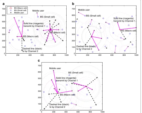
To begin with, we illustrate the eﬀectiveness of the algo-rithm by some examples with randomly generated small cell BS and users, as shown in Figures 4 and 5. To have readable graphical representation and comparison of the user association, channel allocation and transmission power before and after optimization, in these examples, we consider that the path-loss is simply distance depen-dent without log-normal shadowing. So, a user who is farther from a BS has a larger path-loss due to the larger distance. A line connecting a BS and a user indicates the user association and its thickness represents the strength of the transmit power. In these examples, we consider that there are two orthogonal channels in each BS, which are represented by diﬀerent colors and line styles.

Our simulations show that the proposed solution signif-icantly outperforms the by-default conﬁguration in both system throughput (in b/s/Hz) and power consumption eﬃciency (in b/s/Hz/W). Note that the latter has been improved by several orders of magnitude (also because our representation of the default operation has no power control mechanism). Figure 6 shows the corresponding convergence of the algorithm in the above three exam-ples. We see that the algorithm usually converges in a few hundreds of iterations and is hence practical.

4.2 Average performance

Secondly, we compare the performance of the proposed optimization with the default operation, with a fixed num-ber of 32 BS (including the two macro BS) but with different numbers of users (denoted byM), i.e., different user densities, and different numbers of orthogonal chan-nels (denoted byK). Users and small cells are randomly generated in the geographical area. For each(M,K), 500 different topologies are sampled and the performance metrics are then averaged out.

Table 1 shows the the enhancement of the system throughput and of the power eﬃciency obtained by the joint optimization. Observe that for a givenM/Kratio, the spectrum utilization eﬃciency that results from the opti-mization increases withK. This observation is important for e.g., in 3GPP HSDPA (High Speed Downlink Packet Access) and LTE, where a high number of users and a high number of resources are typical.

5 Evaluation of overhead traﬃc

The aim of this Section is to evaluate the overhead traf-fic generated by the algorithms in a specitraf-fic scenario which is based on the assumption that nodes form real-izations of Poisson point processes in the Euclidean plane. These assumptions allow us to use elementary stochastic geometry to get estimates of this overhead traffic.

(8)

0 200 400 600 800 1000 0

100 200 300 400 500 600

700 BS (Macro cell) BS (Small cell)

Mobile user Mobile user

BS (Small cell)

Solid line (magenta): transmit by Channel 1

BS (Macro cell)

Dashed line (black): tx by Channel 2

0 200 400 600 800 1000 0

100 200 300 400 500 600 700

BS (Small cell) Mobile user

BS (Macro cell)

0 200 400 600 800 1000 0

100 200 300 400 500 600 700

Mobile user

BS (Small cell)

BS (Macro cell) Solid line (magenta): transmit by Channel 1

a

b

c

Figure 4Network before optimization (default operation).(a)Example 1: users are concentrated and fewer than BS.(b)Example 2: users are distributed and fewer than BS.(c)Example 3: more users than BS. Performance measure:i)system throughput, andii)power eﬃciency. There are two orthogonal channels represented by solid-magenta and dashed-black lines.

associated with their closest or best base station. The overhead traffic has two main components: (i) the uplink radio traffic and (ii) the backhaul traffic.

5.1 Setting

The uplink radio overhead traﬃc is comprised of the set of messages that are sent by each mobile to its serving base station and that inform the latter of the path-loss that it experiences from each of its neighboring base stations. These data are required to run the algorithm, see e.g., (9). If one denotes by τ the frequency of the beaconing sig-nals from the base stations and if one assumes that the users report their path-loss variables at each beacon, each mobile has to reportN×τpath-loss per second when the number of its neighboring base stations isN.

On the other hand, the backhaul traﬃc is between base stations (it is typically transported by a wireline infrastruc-ture). We will say here that two base stations are neighbors if one of them has customers which see the other as a neighboring base station.

Consider a pair of neighboring base stations. Let M1 denote the number customers of the ﬁrst base station (say BS 1) which see the second (say BS 2) as a neighboring base station. Let M2 be the symmetrical variable. Then the global backhaul traﬃc between the two stations is given by:

M1

i=1 τN1,i+

M2

j=1

(9)

0 200 400 600 800 1000 0

100 200 300 400 500 600 700

Mobile user

BS (Small cell)

BS (Macro cell) BS (Macro cell)

0 200 400 600 800 1000 0

100 200 300 400 500 600

700 _{Mobile user}

BS (Small cell)

BS (Macro cell)

0 200 400 600 800 1000 0

100 200 300 400 500 600 700

BS (Small cell) Mobile user

BS (Macro cell)

a

b

c

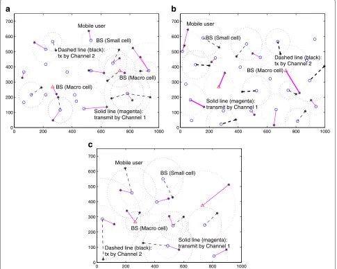
Figure 5Network after proposed joint optimization.Both the system throughput (b/s/Hz) and power utilization eﬃciency (b/s/Hz/W) are signiﬁcantly improved.

whereN1,i denotes the number of neighboring base sta-tions of BS 1 for user iandN2,j denotes the number of neighboring base stations of BS 2 for userj. Note that their deﬁnitions are symmetric.

5.2 Stochastic geometry model

We ﬁrst describe the model for the overhead traﬃc for a purely macro cellular network and then for an heteroge-neous network with both macro and small cells.

5.2.1 Macro cell model

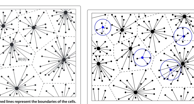
The base stations are assumed to form a Poisson point process of intensityλmin the Euclidean plane. The users are assumed to form an independent Poisson point pro-cess of intensityλuin the Euclidean plane. The association of the users to the closest BS makes the association region

of a base station to be the Voronoi cell of this base sta-tion with respect to the collecsta-tion of base stasta-tions. This association together with the downlinks are depicted in Figure 7.

The mean number of users of a typical cell, denoted by M, is equal toλ_u/λ_m. In our model, we will assume that all users in a cell have for neighboring base stations

Table 1 User average throughput: b/s/Hz, power eﬃciency: b/s/Hz/W

Default After Performance operation optimization gain (times)

M=32,K=1 0.245, 0.0143 1.216, 1.937 4.96, 135

M=64,K=2 0.312, 0.0186 1.583, 2.685 5.07, 144

M=96,K=3 0.356, 0.0210 1.829, 3.149 5.14, 150

(10)

50 100 150 200 250 300 0

50 100 150 200 250

Time iterations (t)

Global energy (

ε

)

(c) Example 3 (a) Example 1 (b) Example 2

Figure 6Convergence of the algorithm: (a) Example 1, (b)Example 2, and(c)Example 3, respectively.

the Delaunay neighbors of the base station which is the nucleus of the cell. This is depicted in Figure 8.

The mean number of Delaunay neighbors of a typi-cal node is 6 and its coeﬃcient of variation CV(N) = √

Var(N)/E(N)isCV(N)=0.222 (see e.g., [21]). Hence, a rough estimate of the mean uplink radio over-head traﬃc is:

R≈6τ λu

λ_m. (14)

0

W(0)

Figure 7The dashed lines represent the boundaries of the cells.

The solid lines link from the base stations to the users which they serve.

Figure 8The solid lines represent the Delaunay graph and serve as model for the backhaul network.

This is only an estimate because there is a correlation between the number of users in a cell and the number of neighbors of the nucleus of this cell. We now give an upper bound onRin complement of this estimate.

The second moment of the number of users in a cell is (see [21]):

E(M2)= λu λm +

1.280λ 2 u λ2 m

. (15)

The second moment of the number of neighbors of a cell is given by:

E(N2)=Var(N)+E(N)2=37.7742. (16)

(11)

One can then use the Cauchy-Schwarz inequality to get

Consider now a typical backhaul link, namely a typical Delaunay edge. A rough estimate of the mean backhaul overhead traﬃc on this link is given by:

B=2R≈12τ λu λm

. (18)

The Cauchy-Schwarz inequality can again be used to get an upper-bound.

5.2.2 Macro and small cell model

In this section, we assume that each small cell has a radius of coverage and that all users covered by the small cell are attached to it. We also assume that small cell rarely over-lap. The users not covered by a small cell are attached to the closest macro base station. This is depicted in Figure 9. We assume that the small cell base stations form an independent point process of intensity λs and that the radius of coverage isρ. The mean number of users in a small cell is thus given by:

Ms=λuπρ2 (19)

while the mean number of users attached to a macro cell is given by:

Mm= λu

λ_m −λuλsπρ

2_. ₍₂₀₎

This formula is only valid under that the Boolean model with intensityλ_s and radiusρhas only rare intersections of balls.

We declare neighbors of a macro cell its macro cell neighbors, deﬁned as above, and all small cells whose base station is located in the macro cell in question or in one of its neighboring macro cells.

We declare neighbors of a small cell the base station of the macro cell it is located in and the macro neighbors of the latter as well as the small cells located in these macro cells.

Since the mean number of small cells per macro cell is λs

λm, the mean number of small cells neighbors of a macro cell is:

Ns_m=7λs

λ_m, (21)

while the mean number of macro cells neighbor of a macro cell is still 6.

The mean number of macro cells neighbors of a small cell is 7 and the mean number of small cells neighbor of a small cell is:

Nm_s =7λs λm

. (22)

Thus, the mean uplink radio overhead traﬃc on a macro cell is given by:

whereas that on a small cell is given by:

Rs ≈ 7τMm+Nms Ms

The mean backhaul traﬃc on a link between two macro base stations is 2Rm, whereas that between a macro base station and a small base station is equal toRm+Rs.

These mean values can be complemented by bounds using second moments.

6 Conclusion

In this article, we analyzed the problem of radio resource allocation in heterogeneous cellular networks composed of macro and small cells with unpredictable cell and user patterns. To solve the problem, we proposed a joint opti-mization of channel selection, user association and power control. The proposed solution, which is based on the Gibbs sampler, is implementable in a distributed manner and nevertheless achieves minimal system-wide poten-tial delay, regardless of the inipoten-tial state. We investigated its performance and estimated the expected overhead. Simulation result and comparison to today’s default oper-ations have shown its high eﬀectiveness in terms of energy consumption. Because of its operational simplicity, this distributed optimization approach is expected to play an important role in the future of heterogeneous wireless networks.

Competing interests

The authors declare that they have no competing interests.

Acknowledgements

(12)

Author details

1_{Network Technologies, Alcatel-Lucent Bell Labs, Centre de Villarceaux, 91620}

Nozay, France.2_{Research group on Network Theory and Communications} (TREC), INRIA-ENS, 75214 Paris, France.

Received: 15 February 2012 Accepted: 25 July 2012 Published: 23 August 2012

References

1. LC Schmelz, JL van den Berg, R Litjens, K Zetterberg, M Amirijoo, K Spaey, I Balan, N Scully, S Stefanski, inWireless World Res. Forum Meeting 22 Self-organisation in wireless networks - use cases and their interrelations, (Paris, France, 2009), pp. 1–5

2. S Sesia, I Touﬁk, M Baker,LTE—The UMTS Long Term Evolution: From Theory to Practice, 2edn. (John Wiley & Son, New York, 2011)

3. CS Chen, F Baccelli, inIEEE International Conference on Communications. Self-optimization in mobile cellular networks: power control and user association (Cape Town, South Africa, 2010), pp. 1–6

4. Z Hasan, H Boostanimehr, V Bhargava, Green cellular networks: a survey, some research issues and challenges. IEEE Commun. Surv. Tutor.13(4), 524–540 (2011)

5. S Saunders, S Carlaw, A Giustina, RR Bhat, VS Rao, R Siegberg,Femtocells: Opportunities and Challenges for Business and Technology(John Wiley & Sons, New York, 2009)

6. 3GPP TS 36942, Evolved universal terrestrial radio access (EUTRA): radio frequency system scenarios. Tech. spec. v10.2.0 (2011)

7. ZQ Luo, S Zhang, Dynamic spectrum management: complexity and duality. IEEE J. Sel. Top. Signal Process.2(1), 57–73 (2008)

8. CS Chen, KW Shum, CW Sung, Round-robin power control for the weighted sum rate maximisation of wireless networks over multiple interfering links. Europ. Trans. Telecommun.22(8), 458–470 (2011) 9. N Ahmed, S Keshav, SMARTA, inACM CoNEXTa self-managing

architecture for thin access points (Lisbon, Portugal, 2006), pp. 1–12 10. I Broustis, K Papagiannaki, SV Krishnamurthy, M Faloutsos, V Mhatre, in

ACM MobiComMDG measurement-driven guidelines for 802.11 WLAN design (Montreal, Canada, 2007), pp. 254–265

11. M Chiang, CW Tan, DP Palomar, D O’Neill, D Julian, Power control by geometric programming. IEEE Trans. Wirel. Commun.6(7), 2640–2651 (2007)

12. CS Chen, GE Øien, inIEEE International Symposium on Wireless Communication Systems. Optimal power allocation for two-cell sum rate maximization under minimum rate constraints (Reykjavik, Iceland, 2008), pp. 396–400

13. L Qian, YJ Zhang, J Huang, MAPEL: achieving global optimality for a non-convex wireless power control problem. IEEE Trans. Wirel. Commun.

8(3), 1553–1563 (2009)

14. S Geman, D Geman, Stochastic relaxation Gibbs distributions, and the Bayesian restoration of images. IEEE Trans. Pattern Anal. Mach. Intell.

PAMI-6(6), 721–741 (1984)

15. P Br´emaud,Markov Chains: Gibbs Fields, Monte Carlo Simulation, and Queues(Springer Verlag, Berlin, 1999)

16. L Massouli´e, J Roberts, Bandwidth sharing: objectives and algorithms. IEEE/ACM Trans. Netw.10(3), 320–328 (2002)

17. P Coucheney, B Gaujal, C Touati, inIEEE PIMRCSelf-optimizing routing in MANETs with multi-class ﬂows (Istanbul, Turkey, 2010), pp. 2751–2756 18. JS Liu, WH Wong, A Kong, Covariance structure and convergence rate of

the Gibbs sampler with various scans. J. Royal Stat. Soc. Ser. B. (Methodological).57(1), 157–169 (1995)

19. 3GPPTS 36331, Evolved universal terrestrial radio access (EUTRA) radio resource control (RRC): protocol speciﬁcation. Tech. spec. v10.4.0 (2011)

20. IEEE 80220 Working Group on Mobile Broadband Wireless Access, Channel models document. 3GPP–3GPP2 Tech. Rep (2007)

21. J Møller,Lectures on Random Voronoi Tessellations(Springer-Verlag, New York, 1994)

22. CS Chen, F Baccelli, L Roullet, inIEEE 73rd Vehicular Technology Conference (VTC Spring)Joint optimization of radio resources in small and macro cell networks (Budapest, Hungary, 2011), pp. 1–5

doi:10.1186/1687-1499-2012-273

Cite this article as: Chen and Baccelli:Gibbsian method for the

self-optimization of cellular networks.EURASIP Journal on Wireless

Communica-tions and Networking20122012:273.

Submit your manuscript to a

journal and beneﬁ t from:

7Convenient online submission 7Rigorous peer review

7Immediate publication on acceptance 7Open access: articles freely available online 7High visibility within the ﬁ eld

7Retaining the copyright to your article