SOLUTION OF A GROUNDWATER CONTROL PROBLEM WITH IMPLICIT FILTERING
A. BATTERMANN
, J. M. GABLONSKY
, A. PATRICK
, C. T. KELLEY
, K. R. KAVANAGH
, T. COFFEY
,AND C. T. MILLER
Abstract. In this paper we describe the application of a parallel implementation of the implicit filtering algorithm
to a control problem from hydrology. We seek to control the temperature at a group of drinking water wells by placing barrier wells between the drinking water wells and a well that injects heated water from an industrial site.
Key words. Implicit filtering, Groundwater flow and transport, Optimal control, Parallel algorithms
1. Introduction. The objective of this paper is to show how the implicit filtering algorithm [11, 15] for noisy optimization problems can be applied to optimization problems in hydrology. We focus on a groundwater temperature control problem. This problem has some of the impor-tant difficulties, such as nonconvexity and nonsmoothness, that one would expect in more difficult cases, but can use flow and transport models and formulations of the optimization problem that are sufficiently simple to allow for a complete description in a single paper. More difficult problems, with coupled flow and transport, temperature dependent densities and viscosities, three dimen-sional geometries, and more complex flow and transport equations, will be considered in future work.
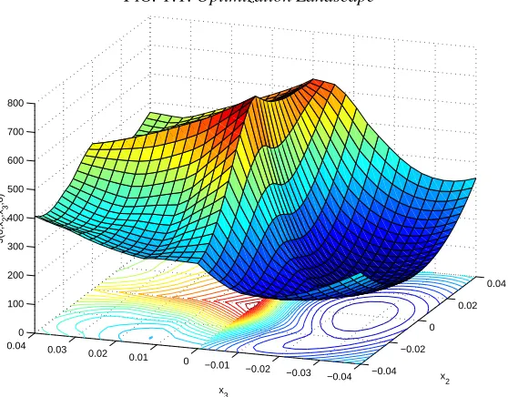
In this paper, we solve the subsurface flow control problem with a parallel implementation [3] of the implicit filtering algorithm [10, 11, 15]. Implicit filtering is a sampling method for optimiza-tion of noisy funcoptimiza-tions. The problem has simple bound constraints and four optimizaoptimiza-tion variables. The objective function is nonconvex, nonsmooth, and has several local minima. The optimization landscape in Figure 1.1 is a plot of the objective function with two of the variables set to zero.
We begin in
2 by briefly discussing the groundwater flow and transport models used in this work and by formulating the control problem.
In
3 we review the implicit filtering algorithm and its implementation in parallel. Then in
4 we report on the results of the optimization and the parallel performance.
2. Groundwater Temperature Control. The problem we consider in this paper was given to us by TGU (Technologieberatung Grundwasser und Umwelt) GmbH, a consulting engineering company for groundwater and water resources. We wish to control the temperature in a set of drinking water wells. The site shown in Figure 2.1 is in the recharge region for these wells. There is an industrial zone on the right of the shaded region which injects heated water in a single well,
Version of December 15, 2000.
Universit¨at Trier, Fachbereich IV, Abteilung Mathematik, 54286 Trier, Germany ([email protected]). This author was supported by the foundation Stiftung Rheinland–Pfalz f¨ur Innovation.
North Carolina State University, Department of Mathematics and Center for Research in Scientific Computation, Box 8205, Raleigh, N. C. 27695-8205 ([email protected], [email protected], [email protected], Tim [email protected], [email protected]). This research was partially supported by National Science Foun-dation grants #DMS-0070641 and #DMS-9714811, Army Research Office grant #DAAD19-99-1-0186, a US Depart-ment of Education GAANN fellowship. Computing activity was partially supported by an allocation from the North Carolina Supercomputing Center.
FIG. 1.1. Optimization Landscape
−0.04 −0.02
0 0.02
0.04
−0.04 −0.03 −0.02 −0.01 0 0.01 0.02 0.03 0.04
0 100 200 300 400 500 600 700 800
x
2
x3
J(0,x
2
,x3
,0)
the infiltration well. German law (the Wasserhaushaltsgesetz) requires that anthropogenic changes of groundwater properties be minimized. In this regulation is the requirement that drinking water be provided at the lowest temperature that is possible under undisturbed conditions. We seek to reduce the temperature at the drinking water wells by minimizing a quadratic function involving pumping rates at a set of barrier wells, which is an approximate measure of cost, and a linear combination of pumping rate and temperature at a set of drinking water wells.
Figure 2.2 shows the relative locations of the wells. The injection well is the square at the far right, the barrier wells the vertical row in the middle, and the drinking water wells are the array on the left.
Numerical experiments show that a steady-state solution is obtained after eight to ten years of real time. Because of this we may use the four steady state pumping rates as control variables. For the work reported here we neglect the vertical dimension and the dependence of viscosity and density on temperature. These assumptions enable us to decouple the equations for flow and temperature and to use a two-dimensional simulator for each. Given the controls, we can solve for the flow and use the results from the flow code to compute the temperature distribution.
To determine the flow we compute the piezometric head from
(2.1)
and appropriate initial/boundary conditions. In (2.1),
is the storage coefficient,
"!$#
is the
thickness of the aquifer, "!$#
is the hydraulic conductivity, and is a source term. From the
head we compute the mean macroscopic pore velocity vector via
%
'&
(
!
(2.2)
where(
is the effective porosity of the porous medium.
FIG. 2.1. Map of the Site
FIG. 2.2. Well Locations
Infiltration well Drinking water well
Barrier well
The water temperature) satisfies *+,) +-/. 01234150 )7698;: 150 )=< (2.3)
where the thermal retardation factor is
*
.
>@?BA$CEDFCEGHC A$IJDKILGMION
(2.4)
In (2.3), A$I
.
P
N
Q
is the volume fraction of the aqueous phase,ARC
.
P
N
S
is the volume fraction of the solid phase,DFC$GJC
.
>
N
TKU'V,WYXZ\[
is the heat capacity of the soil, andDKIHGJI
.
]
N
>^TK_`U'V,WYXZ\[
is the heat capacity of the fluid. For saturated flow,A
.
A$I .
The thermal dispersion tensor is
acbed
.
fg\h
:
hi bjd
? 2 f,k 8 fg 6ml b l d h : h < (2.5)
wherei bed
is the Kronecker i
, and f,k
.
>nPoX
andfg
.
>^X
are longitudinal and transversal disper-sivity values that are characteristic of the porous medium.
3
is a nonsmooth function of: , and
hence ofp . This accounts for the nonsmoothness that is clearly visible in Figure 1.1.
We formulate the optimization problem as
qsrut vnw^x V 2 py6 . pzp ?{ z,) N (2.6) Here p}| *7~
is the vector of steady-state pumping rates at the control wells, ) | *7~
is the temperature at the drinking water wells, and
{ . 2 N PoQK`_ < N P>`>^ < N
P ]`] P
<
N
P ]` > 6z|
*
~
is a vector of the relative pumping rates (inXZJW`n
G ) at these wells. The truncation error in the flow
and transport codes contribute low-amplitude noise to V
.
The bound constraints were imposed to account for limits in the pumping rates. These con-straints were not active at the solution, and the optimization was essentially an unconstrained problem.
3. Implicit Filtering. Implicit filtering [11, 15] is a projected quasi-Newton iteration which uses difference gradients, reducing the difference increment as the optimization progresses. The method was designed for problems with objective functions that are small perturbations of smooth
functions. Our paradigm is
. C ? (3.1) where
C is smooth, and h 2
6
h
is small. In practice
is usually nonsmooth and sometimes discon-tinuous.
Implicit filtering is a sampling method. This means that the optimization is directed only by information on function values, with no gradient information. Implicit filtering differs from classical sampling methods such as the Nelder-Mead [17] or Hooke-Jeeves [12] algorithms in that it is readily implemented in parallel [3, 4, 6] by simply performing the function evaluations needed for the difference gradient in parallel. The potential for quasi-Newton acceleration [5, 11, 15]
is a feature that other parallelizable sampling methods, such as the PDS method [8, 19, 20] or DIRECT [9, 13, 14], cannot exploit. The results reported in this paper were obtained with IFFCO, a FORTRAN implementation of implicit filtering [3].
Suppose we seek to solve su
^Lsy (3.2) where E¡¢9£'y¤¢¥£§¦¥¢©¨Fª (3.3) Here, ¡¢©¨ ¢¬«y and ¦¥¢®¨ ¢¯«y
are sequences of real numbers such that
°7± ² ¡³¢ ² ¦¥¢ ²µ´ ± ª (3.4)
Here we denote the¶th component of the vector
by
y¢
to distinguish the component index from the iteration index. We denote by· the¸¹ projection onto
. For º»7¼ · y¢ ½¾ ¿ ¾À ¡³¢ if y¢¥£µ¡³¢ y¤¢ if ¡¢ ² y¢ ² ¦¥¢ ¦9¢ if y¢¥Á§¦9¢ (3.5)
Implicit filtering as implemented in IFFCO begins by scaling
to the unit cube (
¡¢ ÃÂ
and
¦¥¢ ÅÄ
for all ¶ ). For
Â
²BÆ
£
Â
ªÈÇ
, let ÉËÊ
denote the finite difference approximation of É
with step size Æ
that uses central differences if all points of the central difference stencil are in
and one-sided differences in those directions in which one point in the stencil is not in
. The restrictionÆ
£ÃªÌÇ
implies that at least two points will be in the stencil in any coordinate direction (the center and at least one of
ÎÍ
Æ,Ï , where Ï is the unit vector in that direction). The stencil is
used both to approximate the gradient and to provide one of the termination criteria. Let Ð "Ñ
Æ
be the difference stencil about
in
with step sizeÆ . We call the condition
yÒ£ su ÓR^ÔKÕÖ^× ÊJØ ÚÙK (3.6)
stencil failure. In the unconstrained case [2, 15] stencil failure implies thatÉ YÛ
§Ü
Æ
. A similar result also holds in the bound constrained case, where stencil failure implies that
° · ° É YÛJ yÝ §Ü Æ Mª
We terminate the quasi-Newton iteration for a given value ofÆ
after a stencil failure for this reason. IFFCO offers a choice of SR1 and BFGS quasi-Newton updates. For bound constrained prob-lems we recommend the SR1 update. We will formally describe the algorithm. We begin with Algorithm fdquasi, which is a finite difference projected quasi-Newton iteration for (3.2).
Implicit filtering is a sequence of calls to fdquasi with the difference increments or scales reduced after each return from fdquasi.
There are several convergence theorems for implicit filtering [5, 11, 15]. We state a typical result from [15] for completeness.
THEOREM 3.1. Let
satisfy (3.1) and let É YÛ
be Lipschitz continuous. LetÆÞàß
 , Þ ¨ be the implicit filtering sequence, and Ð
Þ Ð "Ñ ÆÞ
. Assume that fewer than áKâãá
backtracks are taken for all but finitely manyä . Then if
Algorithm 1 fdquasiòó"ôMõôö,÷ãø`ó"ô$ùôMúûô\øK÷ãø`óyü öþýÃÿ
whileö;ö÷ãøKó and \ó ò ó mõòóyü$ü ùOú do
computeõ and5õ
if (3.6) holds then
terminate and report stencil failure end if
update the model Hessian if appropriate; solve ýYõò óyü
use a backtracking line search, with at mostøF÷ãø`ó backtracks, to find a step length
iføK÷ãø`ó backtracks have been taken then
terminate and report line search failure end if
ó ò óü
ö öµÿ
end while
ifö/ö,÷ãø`ó report iteration count failure
Algorithm 2 imfilterò ó"ôMõOô®ö,÷ãø`ó"ô$ùôYú "!Fô\øK÷ãøKóyü
for#sý%$ô'&(&'& do
fdquasiòó"ôMõô®ö÷ãøKó"ôÝùôMú)5ô\øK÷ãøKóyü
end for
then any limit point of the sequence nó*"! is a critical point ofõ"+ .
The implicit filtering method has many parameters, the sequence of scales, the termination parameterù , and the limitsøK÷ãø`ó andö,÷ãø`ó on the inner and outer iterations. We will discuss our
settings of those parameters in , 4.
The most significant opportunity for parallelism is in the computation of 5õ , where all the
function evaluations for ó.-0/=ò ó"ôMúOü are independent. One can also perform the line search
func-tion evaluafunc-tions in parallel. In , 4.2 we show how the parallelism can be effectively exploited by
IFFCO.
4. Computational Results. The computations reported in this section were done on the IBM SP/2 supercomputer located at the North Carolina Supercomputer Center running IBM AIX 4.3. This IBM SP/2 consists of 180 nodes, where each node consists of four 375 MHz Power3-II processors. Each node has 2 GB of memory. We used the IBM xlf 7.1 FORTRAN compiler.
The parameters in the implicit filtering algorithm were ùý ÿ , øK÷ãø`ó ý 1 , ö,÷ãø`ó ý ÿ'$ , 243
ý5&6$"7 for89ý'ÿ`ô'&(&'&Lô97 , and:
3
ý;&6$<7 for89ýÿ`ô'&'&'&Hô97 . We used the SR1 quasi-Newton method
and imposed a limit of 50 function evaluations on the optimization. The scales were ú
3
ý>=@?
3
for ÿA8AB . We terminated the optimization after we expended the budget of 50 function
evaluations.
The parallelism was in the simultaneous evaluations of the objective function to form the difference gradients. We discretized the flow equations on a7C=DE7@= mesh and used MODFLOW
[16] to compute the piezometric head. From the head we extracted the velocity vector and used MT3D [18], a transport simulator, to compute the temperature distribution on the mesh. See [1]
for a more complete account of the model, the boundary conditions, and the underlying physical assumptions. We computed the steady-state solutions using accurate temporal integration out to ten years. For the flow simulation 120 time steps of 30 days are taken. The transport integration was explicit, and we took 150 transport steps for each flow step. MODFLOW and MT3D communicate via disk I/O.
4.1. Effectiveness of the Control. In Figures 4.1 and 4.2 we plot contours of temperature. We normalize the FHG<I9J temperature of the groundwater to zero and the FK<I9J temperature of the
water from the injection well to one. The injection well is located at the box on the right side of the plume, the control wells at the vertical row of diamonds in the center of the plume, and the drinking water wells at the circles to the left of the control wells. The temperature of the injected water isK I J warmer that the ambient groundwater temperature ofF'G I J . This leads to an increase
of F I J at the drinking water wells for the uncontrolled flow, to high satisfy the regulations.
The figures clearly show that the optimized pumping rates reduce the temperature at the drink-ing wells and that the size of the high temperature plume has been reduded. The maximum tem-perature at the drinking water wells is F'GMLNF'I9J for the controlled flow, which is within regulatory
limits.
FIG. 4.1. Temperature Distribution: Uncontrolled Flow
0 0.1 0.2 0.3 0.4 0.5 0.6 0.7 0.8 0.9 1
5 10 15 20 25 30 35 40
5 10 15 20 25 30 35 40
4.2. Parallel Performance. As we described earlier inO 3, there are two opportunities for
par-allelism in IFFCO, the evaluation of the gradient and the line search. We exploit these possibilities in our implementation by using the PVM parallel programming library.
The processors on each node share 2 gigabytes of memory (which did not affect our compu-tations) and a local, temporary directory. We used this temporary directory for the data files and temporary files we needed in our simulation. Since four processors shared the same local direc-tory, we added a unique task identification number (TID) to each each temporary file to prevent the different processors from writing to the same file.
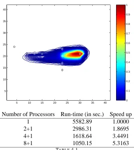
FIG. 4.2. Temperature Distribution: Controlled Flow
0 0.1 0.2 0.3 0.4 0.5 0.6 0.7 0.8 0.9 1
5 10 15 20 25 30 35 40
5 10 15 20 25 30 35 40
Number of Processors Run-time (in sec.) Speed up
1 5582.89 1.0000
2+1 2986.31 1.8695
4+1 1618.64 3.4491
8+1 1050.15 5.3163
TABLE4.1
Paralell efficiency
evaluations. The time needed to do this was much smaller than the time needed to evaluate a function. Therefore, we used the master to run IFFCO and used both the master and the slaves to do the function evaluations needed during the evaluation of the gradient and the line search. We only needed to send short messages between the master and the slaves, so the communication times were very small compared to the computations. This means we only needed to use the basic send and receive mechanisms provided by PVM.
The PVM implementation available on the IBM SP/2 needed a dedicated processor to run the PVM server. In Table 4.1 we show the times needed to solve the problem with different numbers of processors. We record the number of processors as, for example, PRQTS to emphasize that one
processor was needed as the PVM server (a characteristic of the IBM SP/2 PVM). The last column of the table shows the speedup factor U
VXWZY\[
Y
V^]
where
Y\[
is the time needed with one processor and
Y
V
is the time needed with_\Q`S processors.
Perfect speedup for our configuration would be
U
VXW _.
Note that it does not make sense for this problem to use more than nine processors. At most eight processors are required for evaluating the gradient, and one is required as the PVM server. Table 4.1 shows good parallel performance.
REFERENCES
[1] A. BATTERMANN, Mathematical Optimization Methods for the Remediation of Ground Water Contaminations,
PhD thesis, Universit¨at Trier, Trier, Germany, 2001.
[2] D. M. BORTZ ANDC. T. KELLEY, The simplex gradient and noisy optimization problems, in Computational
Methods in Optimal Design and Control, J. T. Borggaard, J. Burns, E. Cliff, and S. Schreck, eds., vol. 24 of Progress in Systems and Control Theory, Birkh¨auser, Boston, 1998, pp. 77–90.
[3] T. D. CHOI, O. J. ESLINGER, P. GILMORE, A. PATRICK, C. T. KELLEY,ANDJ. M. GABLONSKY, IFFCO:
Implicit Filtering for Constrained Optimization, Version 2, Tech. Rep. CRSC-TR99-23, North Carolina
State University, Center for Research in Scientific Computation, July 1999.
[4] T. D. CHOI, O. J. ESLINGER, C. T. KELLEY, J. W. DAVID,ANDM. ETHERIDGE, Optimization of automotive
valve train components with implicit filtering, Optimization and Engineering, 1 (2000), pp. 9–28.
[5] T. D. CHOI ANDC. T. KELLEY, Superlinear convergence and implicit filtering, SIAM J. Optim., 10 (2000),
pp. 1149–1162.
[6] J. W. DAVID, C. Y. CHENG, T. D. CHOI, C. T. KELLEY,ANDJ. GABLONSKY, Optimal design of high speed
mechanical systems, Tech. Rep. CRSC-TR97-18, North Carolina State University, Center for Research in
Scientific Computation, July 1997. Mathematical Modeling and Scientific Computing, to appear in Vol 9.
[7] G.DEMARSILY, Groundwater Hydrology for Engineers, Academic Press, Orlando, 1986.
[8] J. E. DENNIS ANDV. TORCZON, Direct search methods on parallel machines, SIAM J. Optim., 1 (1991),
pp. 448 – 474.
[9] J. GABLONSKY, An implementation of the DIRECT algorithm, Tech. Rep. CRSC-TR98-29, North Carolina
State University, Center for Research in Scientific Computation, August 1998.
[10] P. GILMORE, An Algorithm for Optimizing Functions with Multiple Minima, PhD thesis, North Carolina State
University, Raleigh, North Carolina, 1993.
[11] P. GILMORE ANDC. T. KELLEY, An implicit filtering algorithm for optimization of functions with many local
minima, SIAM J. Optim., 5 (1995), pp. 269–285.
[12] R. HOOKE ANDT. A. JEEVES, ‘Direct search’ solution of numerical and statistical problems, Journal of the
Association for Computing Machinery, 8 (1961), pp. 212–229.
[13] D. R. JONES, The DIRECT global optimization algorithm. to appear in the Encylopedia of Optimization, 1999.
[14] D. R. JONES, C. C. PERTTUNEN, AND B. E. STUCKMAN, Lipschitzian optimization without the Lipschitz
constant, J. Optim. Theory Appl., 79 (1993), pp. 157–181.
[15] C. T. KELLEY, Iterative Methods for Optimization, no. 18 in Frontiers in Applied Mathematics, SIAM,
Philadelphia, 1999.
[16] M. G. MCDONALD ANDA. W. HARBAUGH, A modular three-dimensional finite-difference groundwater flow
model, U.S. Geological Survey Techniques of Water Resources Investigations, Book 6, Ch. A1, Reston, VA,
1988.
[17] J. A. NELDER ANDR. MEAD, A simplex method for function minimization, Comput. J., 7 (1965), pp. 308–313.
[18] S. S. PAPADOPULOS, MT3D: A modular three-dimensional transport model, Version 1.5, Documentation and
User’s Guide, S. S. Papadopulos & Associates, Inc., Bethesda, Maryland, 1992.
[19] V. TORCZON, On the convergence of the multidimensional direct search, SIAM J. Optim., 1 (1991), pp. 123–
145.