Analysis of Inflection and Singular Points on Parametric Curve with a Shape Factor

(1)

Article

Analysis of Inflection and Singular Points on Parametric Curve

with a Shape Factor

Zhi Liu 1,_{*, Chen Li}2_{, Jieqing Tan}1_{and Xiaoyan Chen}1

1 _{School of Mathematics, Hefei University of Technology, Hefei 23009, China;} [email protected] (J.T.); [email protected] (X.C.)

2 _{College of Information & Network Engineering, Anhui Science and Technology University, Chuzhou 233100, China;} [email protected]

* Correspondence: [email protected]

Abstract: The features of a class of cubic curves with a shape factor are analyzed by means of the theory of envelope and topological mapping. The effects of the shape factor on the cubic curves are made clear. Necessary and sufficient conditions are derived for the curve to have one or two inflection points, a loop or a cusp, or to be locally or globally convex. Those conditions are completely characterized by the relative position of the edge vectors of the control polygon and the shape factor. The results are summarized in a shape diagram, which is useful when the cubic parametric curves are used for geometric modeling. Furthermore we discussed the influences of the shape factor on the shape diagram and the ability for adjusting the shape of the curve.

Keywords: shape factor; singular points; inflection points; local convexity; global convexity

1 Introduction

Bézier curves and surfaces are modeling tools widely used in CAD/CAM systems [1]. The use of Bernstein polynomials as the basis functions in Bézier’s UNISURF is well known. Cubic Bernstein basis functions are

{

₍₁

₋

_u

_{) , 3(1}

3

₋

_{u u}

_{) , 3 (1}

2

_u

2

₋

_{u u}

_),

3

}

_.

In the CONSURF system developed by A A Ball [2-4] at the British Aircraft Corporation, the following basis for cubic polynomials was used

{

₍₁

₋

_u

_{) , 2(1}

2

₋

_{u u}

_{) , 2 (1}

2

_u

2

₋

_{u u}

_),

2

}

_.

Said [5] extended it to arbitrary odd degrees, namely the generalized Ball curves. The generalized Ball curves possess many nice properties which are similar to those of Bézier curves, such as, computational stability, symmetry property, convex hull property, endpoint interpolation, geometric invariant [6]. The generalized Ball representations for a polynomial curve are much better suited to degree raising and lowering than Bézier representations. It is well known that degree elevation and reduction are important in transferring data between various CAD systems. Goodman and Said [7,8] suggest that, in the situation where degree elevation and reduction are important, while other process are less important, the designer of curves and surfaces should consider using the generalized Ball form instead of the Bézier form.

In CAD/CAGD, it is often necessary to detect inflection points and singularities on curves. Convexity is an important intuitive geometric concept and convexity control of curves and surfaces plays a fundamental role. For planar cubic Bézier curves an exhaustive study was presented in [9] and for the rational case in [10]. Manocha [11] studied this problem for polynomial and rational parametric curves of arbitrary degree. Yang [12] discussed inflection points and singularities on C-Bézier curves, and the results are summarized in a shape diagram of C-Bézier curves. Juhász [13] detected cusps, inflection points and loops of C-Bézier curves by letting a control point vary while the rest is held fixed. But locally and globally convex is not referred to. There are many other publications on this topic [14].

(2)

This paper is organized as follows: First we show the construction of a class of cubic parametric curves with a variable shape factor. Ball curve, cubic Bézier curve and cubic Timmer curve are special cases of the curve. In Section 3, the inflection points and singularities of the space cubic parametric curves are discussed. In Section 4, shape features of the planar cubic parametric curves are proposed by using the method based on the theory of envelope and topological mapping. Necessary and sufficient conditions are derived for this curve to have one or two inflection points, a loop or a cusp, to be locally or globally convex. The results are summarized in a shape diagram. At last, the influences of shape factor on the shape diagram and their ability for adjusting the shape of the curve are analyzed.

2 The cubic parametric curve with a shape factor

Definition 2.1. Given four control points d

(

2,3,

0,1, 2,3)

i

∈

d

=

i

=

P

R

, the cubic parametric curve with a

shape factor is defined as follows

[ ]

3

0

( )

i i

( ) ,

0,1 ,

i

t

B t

t

=



∈

p

P

(1)

where

B t i

_i

( )(

=

0,1, 2,3)

are the basis functions with the shape factor

λ

defined by

2 2

0 1

2 2

2 3

( ) [1 (2

) ](1

) ,

( )

(1 ) ,

( )

(1

),

( ) [1 (2

)(1 )] .

B t

t

B t

t

B t

t

B t

t t

λ

= + −

−

=

−

=

−

= + −

−

(2)

If

λ

=

0

, the cubic parametric curve degenerates into a straight line. If

λ

=

2

, the cubic parametric curve degenerates into Ball curve. If

λ

=

3

, the cubic parametric curve degenerates into cubic Bézier curve. If

λ

=

4

, the cubic parametric curve degenerates into cubic Timmer curve [16]. So, Ball curve, cubic Bézier curve and cubic Timmer curve are all special cases of the cubic parametric curve defined in (1).

When parameter

_λ

_∈

(

0,3

]

, The cubic parametric curves have similar properties to cubic Bézier curve or Ball curve, such as symmetry, the endpoint interpolation, end edge tangent, convex hull property and geometrical invariance etc. And the cubic parametric curve also has a similar recursive evaluation, degree elevation and reduction algorithms. So we assume that

_λ

∈

(

0,3

]

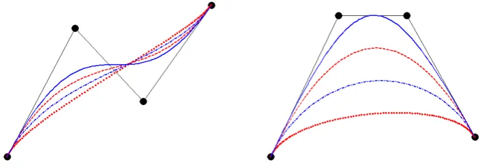
in this paper.

The introduction of the variable shape factor makes the curve shape feature distribution simpler and easier to control. Given four control points, we can globally or locally adjust the shape of curve by changing the shape factor value. The cubic parametric curve is more approximate to the control polygon with the increasing shape factor

λ

, otherwise away from the control polygon. Therefore the cubic parametric curve is more flexible in adjusting the shape of the curve than either cubic Bézier curve or Ball curve.

Fig. 1 shows the cubic parametric curves with shape factor

λ

=

1

,

λ

=

2

(Ball curve),

λ

=

3

(cubic Bézier curve) and

λ

=

4

(cubic Timmer curve), respectively.

Fig. 1. The cubic parametric curves with a shape factor (red dotted lines,

λ

=

1

; blue dash dotted lines,

λ

=

2

; red dashed lines,

λ

=

3

; blue solid lines,

λ

=

4

)

3 Geometric features of the space cubic curve

(3)

Theorem 1. If _λ_∈(0, 3] and the control points

P

_i

∈

R

3

(

i

=

0,1, 2,3

)

are not coplanar, then the cubic parametric curve

p

( )

t

has no singular point, cusp, double point or pan inflection point, and the direction of rotation of the curve

p

( )

t

is consistent with that of the control polygon.

Proof: First, we prove that the curve

p

( )

t

has no cusp.Let

q

_i

= −

P P

_i _i₋₁

(

i

=

1, 2,3

)

be the edge vectors of the control polygon. Then

p

( )

t

can be simplified to

0 0 1 2 3 2 3 3

( )

t

=

+ −

[1

B t

( )]

+

[ ( )

B t

+

B t

( )]

+

B t

( ) .

p

P

q

(3)

Therefore,

0 1 2 3 2 3 3

( )

t

B t

( )

[ ( )

B t

( )]

B t

( )

′

= −

′

+

′

+

′

+

′

p

q

.

When

t

_∈

(0,1)

, it follows from (2)

2

( )

3

( ) 6 (1

) 0

B t

′

+

B t

′

=

t

− ≠

t

.

Since the control points

P

_i

(

i

=

0,1, 2,3)

are not coplanar, the edge vectors

q

_i

(

i

=

1, 2,3

)

are linearly independent, so

p

_{′ ≠}

( )

t

0

. Therefore the curve

p

( )

t

has no cusp.

Next, we prove that the curve

p

( )

t

has no double point. Assume that the curve

p

( )

t

has a double point, say,

1 2

( )

t

−

( ) 0

t

=

p

, where

0 ≤ < ≤

t

₁

t

₂

1

. Then it follows from (3)

[

B t

0

( )

2

−

B t

0 1

( )

] [

q

1

+

B t

2 1

( )

+

B t

3 1

( )

−

B t

2

( )

2

−

B t

3

( )

2

] [

q

2

+

B t

3 1

( )

−

B t

3

( )

2

]

q

3

=

0

.

Since the edge vectors

q

i

(

i

=

1, 2,3

)

are linearly independent, we have

B t

i

( )

1

=

B t

i

( ),

2

i

=

0, 2,3.

B t

₀

( )

₁

=

B t

₀

( )

₂ implies that there exists

_ξ

∈

( , ) [0,1]

t t

₁ ₂

⊆

such that

B

₀

′

( ) 0

_ξ

=

, namely,

3(

2)

λ

ξ

λ

=

−

.

Since

0 < <

_ξ

1

, we have

0

1 3(

2)

λ

<

−

, which results in

λ

>

3

or

λ

<

0

, contradicting

λ

∈

(0,3]

. Therefore

B t

₀

( )

₁

≠

B t

₀

( )

₂ . Hence the curve

p

( )

t

has no double point.

Last, we prove that the curve

p

( )

t

has no pan inflection points, and the direction of rotation of

p

( )

t

is consistent with that of the polygon.

The point

p

( ) 0

t

₀

(

< <

t

₀

1 )

is the pan inflection point of the space curve

p

( )

t

if and only if the sign of torsion changes when it passes through

t

₀. We assume

( ) det( ( )

( ),

( ))

g t

=

P

′

t

, P

′′

t

P

′′′

t

. Note that

3

0

( ) 1

i i

B t

=



,

3 3 3

0 0 0

( )

( ) 0

i i i

B t

= = =

′

=

′′

=

′′′

=



.

Then

3 3 3 3

3 3 3

0 0 0 0

3 3 3 3

0 0 0

0 0 0 0

( )

( ) det

( )

i i i i

i i i i i i

i i i

i i i i i i i i

i i i i

B t

g t

B t

= = = =

= = =

= = = =

′

′′

′′′



_′

_′′

_′′′



=

_

_

=





_′

_′′

_′′′



P

0 0 0 0

1 1 1 1

0 1 2 3 2 2 2 2

3 3 3 3

( )

1

1 ( )

( )

B t

′

′′

′′′







_′

_′′

_′′′





_{ }

_

=

_

_

′

′′

′′′









_

_

′

′′

′′′





(4)

0 0 0 0

1 1 1 1

1 2 3

0 1 2 3 2 2 2 2

3 3 3 3

( )

1

0

0 ( )

( )

( , , ) ( ),

( )

B t

D t

B t

′

′′

′′′

′

′′

′′′

=

_′

_′′

_′′′

=

′

′′

′′′

q q q

P

q

where

( , , )

q q q

₁ ₂ ₃ is the mixed product of the edge vectors

q q q

₁

, ,

₂ ₃. The edge vectors

q q q

₁

, ,

₂ ₃ are not coplanar, so

( , , ) 0

q q q

₁ ₂ ₃

≠

. Since

_λ

∈

(0,3]

，we get

0 0 0 0

1 1 1 1 2

2 2 2 2

3 3 3 3

( )

12

0 ( )

( )

B t

D t

B t

λ

′

′′

′′′

′

′′

′′′

=

_′

_′′

_′′′

=

>

′

′′

′′′

.

For

0 ≤ ≤

t

1

, we have

g t

( ) 0

≠

and

g t

( )

has the same sign as

( , , )

q q q

₁ ₂ ₃ . So the cubic parametric curve

p

( )

t

has no pan inflection point and the direction of rotation of the curve

p

( )

t

is consistent with that of the polygon. The proof of Theorem 1 is completed.

4 Geometric features of the planar cubic curve

It is known that a planar cubic parametric curve may have one or two inflection points, a loop or a cusp. If the control points

P

_i

∈

R

3

(

i

=

0,1, 2,3

)

are coplanar, then edge vectors

q

_i

(

i

=

1, 2,3)

are linearly dependent and the cubic parametric curve

p

( )

t

reduces to a plane curve. The following discussion is based on the positional relationship of

q

₁ and

q

₃.

4.1 Edge vectors

q

₁ and

q

₃ are non-parallel

When edge vectors

q

₁ and

q

₃ are non-parallel,

q

₁ and

q

₃ are the base vectors of the plane. Let

2

=

u

1

+

v

3

q

. From equation (3), we have

(

)

(

)

0 0 2 3 1

3 2 3 3

( )

1 ( )

( )

t

B t

u B t

B t

v B t

B t

=

+ −



_

+



_

+



_

+



_

p

P

q

(4) If

p

′ =

( )

t

0 (0

< <

t

1)

, then

(

)

(

)

0

( )

2

( )

3

( )

1 3

( )

2

( )

3

( )

3

B t

′

u B t

′

B t

′

B t

′

v B t

′

B t

′

−

+

=













q





q

0

. (5)

Since

q

₁ and

q

₃ are linearly independent, we have

0 2 3 3 2 3

( )

:

(0

1)

( )

B t

u

B t

C

t

B t

v

B t



_′

=



′

₊

′



< <



′



= −



_′

+



.

Substituting (2) into the above two equations gives

(

)

1

2

6 :

0 1 .

1

2 6(1

)

u

t

C

t

v

t

λ



_{= − −}



_{< <}





_{= − −}

−



(6)

(5)

0

lim

t→ +

u

= −∞

, t

lim

0

v

3

1 λ

+

→

= −

,

lim

t 1

u

3

1 λ

−

→

= −

,

lim

t→1−

v

= −∞

.

So the curve

C

has two asymptotes:

1,

1

3

3 u

= −

λ

v

= −

λ

. On the other hand, we get from (6)

( )

2 2

d

0 d

₁

v

t

u

= −

_t

₋

<

,

_{( )}

2 3

3 2

d

12

0 d

₁

v

t

u

=

_λ

_t

₋

<

.

Therefore, the curve

C

is monotonic decreasing

(0

< <

t

1,

_λ

∈

(0,3])

and has no inflection point.

By means of the monotone and strict convexity of the curve

C

, we further discuss the cusps, the inflection points and convexity of the curve

p

( )

t

.

4.1.1 About the cusp

The necessary condition for the curve

p

( )

t

to have a cusp is

(

)

( ) 0 0

t

1 ′ =

< <

p

.

Suppose

t

₀

(

0 < <

t

₀

1 )

is the point corresponding to

(

u v

₀

,

₀

)

∈

C

, such that

p

′

( ) 0

t

₀

=

．

The Taylor expansion of

p

( )

t

about

t

₀ is

2 2

0 0 0 0 0 0

1 ( )

( )

( )(

)

( )(

)

(

) .

2 t

=

t

+

′

t t t

−

+

′′

t t t

−

+

ο

t t

−

p

Differentiating the above equation yields

0 0 0

( )

t

( )(

t t t

)

_ο

(

t t

)

′

=

′′

−

+

−

p

,

where

p

′′

( ) 0

t

₀

≠

. In fact, by (5)

p

′′ =

( )

t

0 (0

< <

t

1)

implies

(

)

(

)

0

( )

2

( )

3

( )

1 3

( )

2

( )

3

( )

3

.

B t

′′

u B t

′′

B t

′′

B t

′′

v B t

′′

B t

′′

−

+

=













q





q

0

Since

q

₁ and

q

₃ are linearly independent, we have

0

2 3

3

2 3

( )

(0

1)

( )

B t

u

B t

t

B t

v

B t

′′



₌



_′′

₊

_′′



_{< <}



_′′

−



₌



′′

+

′′



.

That is

1

2 6(2 1)

(0

1)

1

2 6(2 1)

u

t

v

t

λ



_{= − −}



₋



< <





_{= − +}



₋



. (7)

If (6) and (7) hold simultaneously, then we get

_λ

=

0

, contradicting

_λ

_∈

(0,3]

, so

p

′′

( ) 0

t

₀

≠

.

While

p

′

( ) 0

t

₀

=

,

p

′′

( ) 0

t

₀

≠

, we know the direction of

p

′

( )

t

changes when it passes through

t

₀. As a result,

p

( )

t

₀ is a cusp on the curve

p

( )

t

. And therefore the curve

p

( )

t

having cusp is equivalent to

( , )

u v

∈

C

.

4.1.2 About the inflection point

The point

p

( ) 0

t

₀

(

< <

t

₀

1 )

is the inflection point of the curve

p

( )

t

if and only if the direction of

( )

t

( )

t

′

×

′′

p

t

₀. According to equation (4), we have

(

)(

1 3

)

( )

t

( )

t

f t u v

; ,

′

×

′′

=

×

(6)

Where

(

)

0 3 2 3 0 1

2 2 2

( )

; ,

( )

6 (2

)

6 (

2)

2 (3

) 6

6 ( 1) .

B t

f t u v

u

v

B t

t

t u

t

v

λ

λ λ

λ

′

= −

+

′′

=

−

+

−

+

− +

+

−

As a result，

P

( ) 0

t

₀

(

< <

t

₀

1 )

is an inflection point of the curve

p

( )

t

if and only if the sign of

f t u v

(

; ,

)

t

₀. In the uv-plane, the curve

p

( )

t

with the potential region of inflection points shall be covered with a family of straight lines. By the theory of envelope [17], the envelope of the straight lines is

(

)

(

)

; ,

0,

; ,

0.

t

f t u v

=





_′

=



That is

2 2 2

3 (2

)

3 (

2)

(3

) 3

3 ( 1)

0,

2 (2

)

(

2) 2

2 (

1)

0. t

t

t u

t

v

t

tu

t

v

λ

λ λ

λ

λ λ

λ



₋

₊

₋

₊

_{− +}

₊

₋

₌



−

+

− +

+

−

=



(8)

It is not difficult to find that

u

and

v

given by (6) are the solution of equations (8), which means that the envelope of the straight lines is just the curve

C

.

As previously described, the curve

C

is a strictly convex and continuous curve. So the swept region of tangent of the curve

C

is

S D C

 

. That is the potential region of inflection point(s). As shown in Fig. 2, the region

D

is composed of two asymptotes

1,

1

3

3 u

= −

λ

v

= −

λ

and the curve

C

(not including the curve

C

). The region

S

includes two parts: one part is in the upper left part of the intersection of the two asymptotic lines, the other part is the lower right part of that. Given in Fig.2 are three different regional distributions of inflection point(s) corresponding to

_λ

=

1

,

_λ

=

2

and

_λ

=

3

.

a.

_λ

=

1

b.

λ

=

2

c.

λ

=

3

Fig. 2. Regional distribution of inflection point (S, single inflection point region; D, double inflection points region)

For any point

(

u v

₀

,

₀

)

∈

S D C



, at least one line

f t u v

(

₀

; ,

)

=

0

passing through

(

u v

₀

,

₀

)

on uv-plane is tangent to the curve

C

. Suppose

(

u v

₀

,

₀

)

∈

C

corresponds to the parameter

t

₀

.

Then we have

(

0

; ,

0 0

)

0 f t u v

=

and

f t u v

_t

′

(

₀

; ,

₀ ₀

)

=

0

. The Taylor expansion of

f t u v

(

; ,

₀ ₀

)

about

t

₀ is

(

)

(

)(

)

2

(

)

2

0 0 0 0 0 0 0

1 ; ,

; ,

2

tt

f t u v

=

f t u v

′′

t t

−

+

_ο

t t

−

where

(

0 0 0

)

0 0 2

0 0

2 ; ,

12 (2

) 12

12 .

(

1)

tt

f

t u v

u

v

t t

λ

′′

₌

_{− +}

₊

₌

−

(7)

If

(

u v

₀

,

₀

)

∈

S D



, let

f t u v

(

₀

; ,

)

=

0

be the straight line passing through

(

u v

₀

,

₀

)

and be tangent to the curve

C

. The Taylor expansion of

f t u v

(

; ,

₀ ₀

)

about

t

₀ is

(

; ,

0 0

)

t

(

0

; ,

0 0

)(

0

) (

0

)

f t u v

=

f t u v

′

t t

−

+

_ο

t t

−

,

where

f t u v

_t

′

(

₀

; ,

₀ ₀

)

≠

0

(if

f t u v

_t

′

(

₀

; ,

₀ ₀

)

=

0

, then

(

u v

₀

,

₀

)

∈

C

). As a result, the sign of

f t u v

(

; ,

₀ ₀

)

t

₀. That is,

p

( )

t

₀ is the inflection point of the curve

p

( )

t

.

Furthermore, if

(

u v

₀

,

₀

)

∈

S

, then there exists only one straight line that is tangent to the curve

C

and passing through

(

u v

₀

,

₀

)

, and the corresponding cubic parametric curve

p

( )

t

has only one inflection point. If

(

u v

0

,

0

)

∈

D

, then there exist two straight lines that are tangent to the curve

C

and passing through

(

u v

0

,

0

)

,

and the corresponding curve

p

( )

t

has double inflection points.

Fig. 2 shows that double inflection region of Ball curve is smaller than that of the cubic Bézier curve. But single inflection regions of these two kinds of curves are of the same size.

4.1.3 About the double point

The curve

p

( )

t

has a double point if and only if there are

0 ≤ < ≤

t

₁

t

₂

1

such that

1 2

( )

t

−

( ) 0

t

=

p

,

which, according to equation (4), leads to the following system of equations

0 2 0 1

2 2 3 2 2 1 3 1

3 1 3 2

2 2 3 2 2 1 3 1

( )

,

( )

,

( )

B t

u

B t

v

B t

−



₌



₊

₋





₋



₌



₊

₋



(9)

where

(

t t

₁

,

₂

)

∈Δ =

{

(

t t

₁

,

₂

)

∈

R

2

0 ≤ < ≤

t

₁

t

₂

1

}

.

The system of equations (9) defines a topological mapping

F

:

Δ ⊂

R

2

→

F

( )

Δ ⊂

R

2. The image region

( )

L F

=

Δ

is simply connected region on uv-plane. The three boundary lines of region

Δ

:

t

₁

=

t t

₂

,

₁

=

0

and

2

1 t

=

correspond to the three boundary curves of the image region

L

: the curve

C

(does not belong to

L

), the curve

L

₁ and

L

₂ (both belong to

L

), where

2

1

( 1)

1,

(2

3)

:

(0

1),

( 1)

1,

2

3 t

u

t t

L

t

v

t

λ



₋

=

−



−

_{< ≤}



−



₌

₋



₋



2 2

1,

2

1 :

(0

1).

1,

( 1)(2

1)

t

u

t

L

t

v

t

λ



₌

₋



₊



_{≤ <}





₌

₋



₋

₊



For the curve

L

₁,

_λ

_∈

(0,3], 0

_{< <}

t

1

, we know

2

d

0 d

( 1)(

3)

v

t

u

= −

t

−

t

−

<

,

( )

3 2

2

d

2 (2

3)

0 d

1 (

3)

v

t t

u

_λ

t



₋



= ⋅





<

−





, t

lim

_→0+

u

= −∞

, _t

lim

₀

v

₃

1 λ

+

→

= −

.

(8)

2

d

(

2)

0 d

( 1)

v

t t

u

t

+

= −

<

−

,

3 2

2

d

2

1

0 d

1 v

t

u

_λ

t

+





= ⋅

_

_

<

−





,

lim

t 1

u

3

1 λ

−

→

= −

,

lim

t→1−

v

= −∞

.

As a result，both the curves

L

₁ and

L

₂ are monotonically decreasing and strictly convex continuous curves. The curve

L

₁ intersects the curve

L

₂ at the point

( 1, 1)

− −

. What is more, the curve

L

₁ has the asymptote

1

3 v

= −

λ

and the curve

L

₂ has the asymptote

1

3 u

= −

λ

, and the curve

C

does not intersect

L

₁ and

L

₂,

as shown in Fig. 3.

In summary, the curve

C

(does not belong to

L

), and the curves

L

₁ and

L

₂ (both belong to

L

) round into simply connected region

L

. If

(

u v

₀

,

₀

)

∈

L

, the corresponding cubic parametric curve

p

( )

t

has only one double point.

Example. For a given set of control points

P

_i

∈

R

2

(

i

=

0,1, 2,3)

, a few different cubic parametric curves contain singularities can be designed according to the conditions discussed above. Fig. 3 illustrates that the singularity can be removed by changing the value of the shape factor

λ

.

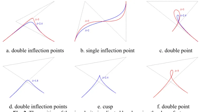
Fig. 3a shows two segment cubic curves containing double inflection points when

_λ

=

2.4

and

_λ

=

3

. Fig. 3b is two segment cubic curves containing a single inflection point. Fig. 3c is two segment cubic curves containing a double point. For the same control polygon, Fig. 3d~f denote cubic curves containing double inflection points, cusp, double point, respectively. In particular, when

_λ

=

3

, the red curve is a cubic Bézier curve in Fig. 3.

a. double inflection points b. single inflection point c. double point

d. double inflection points e. cusp f. double point

Fig. 3. The position of the singularity is adjusted by changing the shape factor

Figure 3 tells us that we can construct the curve with the desired geometric characteristics by adjusting the shape factor value. Cubic parametric curve can construct more abundant geometric characteristics than cubic Bézier curve in geometric design.

4.1.4 Aboutthe convexity

We will discuss the case of

( , )

u v

∈ =

N

R

2

\

(

C S D L

  

)

, meanwhile there are no cusp, double points or inflection points on the cubic parameter curve. And the direction of the binormal vector

p

′

( )

t

×

p

′′

( )

t

does not change.

The upper left part of the area surrounded by the curves

L

₁ and

L

₂ (not including the curves

L

₁ or

L

₂) is marked as

N

₁, and the lower right part of the area surrounded by the curves

L

₁ and

L

₂ is marked as

N

₂. Set

N

₀

=

N

\ (

N

₁



N

₂

)

, as shown in Fig.3.

(9)

1 3

( )

t

=

′

(0) [ ( )

×

t

−

(0)]

=

_ϕ

( ; , )(

t u v

×

)

m

p

q q

, (10)

1 3

( ) [ ( )

t

=

t

−

(0)]

×

′

( )

t

=

_ψ

( ; , )(

t u v

×

)

n

p

q q

. (11) According to equations (4) and (5), we have

{

}

2

[

]

3 2 3

( ; , )

t u v

B t

( )

v B t

[ ( )

B t

( )]

t

(3

) (

2)

t

(3 2 ) .

t v

ϕ

=

λ

+

=

λ

− +

λ

−

+ −

(12)

{

}

{

}

0 3 3 0 2 3 3 2 3 3

0 2 3 0 2 3

( ; , ) [1

( )] ( )

( ) ( )

[ ( )

( )] ( ) [ ( )

( )] ( )

[1

( )][ ( )

( )]

( )[ ( )

( )] .

t u v

B t B t

u B t

B t B t

B t

B t B t

v

B t

B t B t

B t

ψ

= −

′

+

′

+

′

−

′

+

′

+

−

+

(13)

For any

t

₀

∈

(0,1)

, if none of the directions of the vectors

m

( )

t

,

n

( )

t

and

p

′

( )

t

×

p

′′

( )

t

changes when they pass through

t

₀, the curve

p

( )

t

is globally convex. If the direction of the binormal vector

p

′

( )

t

×

p

′′

( )

t

does not change when it passes through

t

₀, but the direction of

m

( )

t

or

n

( )

t

changes, then the curve

p

( )

t

is locally convex [13]．

As described above, if

( , )

u v

∈ =

N

₀



N

₁



N

₂, the sign of the function

f t u v

( ; , )

does not change, and the direction of the binormal vector

p

′

( )

t

×

p

′′

( )

t

does not change.

From equation (12), if

3 0

2 0 3 0 0

( )

1 ( )

( )

2 2(2

3)

B t

v

B t

t

λ

= −

= − +

+

−

,

then

_ϕ

( ; , ) 0

t u v

₀

=

, and the direction of the vector

m

( )

t

₀ and the range of

v

is

1

3 v

λ

− < < −

. And so, if

( , )

u v

∈

N

₁, the direction of either

p

′

( )

t

×

p

′′

( )

t

, or

n

( )

t

does not change

when they pass through

t

m

( )

t

changes, the curve

p

( )

t

is locally convex. In fact,

N

₁

happens to be the area covered by the tangent of

L

₂ in the region

N

. Similarly, solving the equations

( ; , ) 0,

( ; , ) 0.

t

t u v

ψ

=





_′

₌



for

u v

,

verifies that the envelope of the family of straight lines

_ψ

( ; , ) 0

t u v

₌

happens to be the curve

L

₁.If

2

( , )

u v

∈

N

, the direction of either

p

′

( )

t

×

p

′′

( )

t

or

m

( )

t

does not change when they pass through

t

n

( )

t

changes, so the curve

p

( )

t

is locally convex. The region

N

₂ is the area covered by the tangent of

L

₁ in the region

N

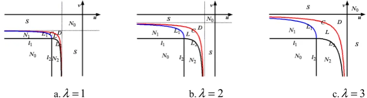
. As shown in Fig. 4, where

l v

₁

:

= −

1 (

u

< −

1 )

and

l u

₂

:

= −

1 (

v

< −

1 )

.

If

( , )

u v

∈

N

₀, none of the directions of

m

( )

t

,

n

( )

t

and

p

′

( )

t

×

p

′′

( )

t

changes when they pass through

0

t

. Therefore the curve

p

( )

t

is globally convex.

a.

_λ

=

1

b.

_λ

₌

2

c.

_λ

=

3

Fig.4. The shape distribution of the cubic parameter curve (C is cusp region; L is double point region; S is single inflection point region; D is double inflection points region; N0 is global convexity region;

N

₁



N

₂ is local

(10)

Theorem 2. When edge vectors

q

₁ and

q

₃ are non-parallel, let

q

₂

=

u

q

₁

+

v

q

₃. Shape features of the plane cubic parametric curve

p

( )

t

depend on the following distribution of points

( , )

u v

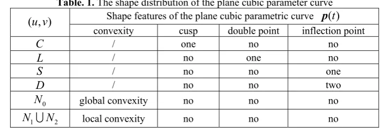
in the uv-plane (As shown in Table. 1).

Table. 1. The shape distribution of the plane cubic parameter curve

( , )

u v

Shape features of the plane cubic parametric curve

p

( )

t

convexity cusp double point inflection point

C

/ one no no

L

/ no one no

S

/ no no one

D

/ no no two

0

N

global convexity no no no

1 2

N



N

local convexity no no no

4.2 Edge vectors

q

₁ and

q

₃ are parallel

If

q q

₁

||

₃, without loss of generality, edge vectors

q

₁ and

q

₂ are the base vectors of the plane. Let

q

₃

=

α

q

₁. From equation (3), we have

[

] [

]

0 0 3 1 2 3 2

( )

t

=

+ −

1 B t

( )

+

_α

B t

( )

+

B t

( )

+

B t

( )

.

p

P

q

(14)

4.2.1 about the cusp

We discuss the curve

p

( )

t

similarly to section 4.1.1. The curve

p

( )

t

having cusp is equivalent to

( ) 0,

t

(0,1)

′ =

∈

p

. From equation (14), we have

[

0 3

] [

1 2 3

]

2

( )

t

B t

( )

_α

B t

( )

B t

( )

B t

( )

′

= −

′

+

′

+

′

+

′

p

q

.

Because edge vectors

q

₁ and

q

₂ are linearly independent, we know

p

′ =

( ) 0,

t

∈

(0,1)

is equivalent to

2 2

[3(

2)

2(3 2 )

]

[3(

2)

2(3

) ] 0

6 (1

) 0

t

λ

λ α λ

λ



₋

₊

₋

_{+ +}

₋

₊

₋

₌



− =



(15)

It is obvious that equations (15) has no solution for

t

in

(0,1)

. So the plane cubic parameter curve

p

( )

t

has no cusp.

4.2.2 About the inflection point

The point

p

( ) 0

t

₀

(

< <

t

₀

1 )

is the inflection point of the curve

p

( )

t

if and only if the direction of

( )

t

( )

t

′

×

′′

p

t

₀. According to equation (14), we have

( )(

1 2

)

( )

t

( )

t

f t

;

_α

′

×

′′

=

×

p

q q

,

where

( )

0 2 3 3 2 3

2 2

( )

;

( )

6 (1

)

.

B t

f t

B t

t

α

λ

α

′

₊

′

₊

′

= −

+

′′

₊

′′

₊

′′





=

_

−

_

When

_α

>

0

,

( )

;

12 (

1 )

0

t

f t

′

_α

=

_λ

t

− −

_α

t

<

. Because

( )

0;

6

0 f

_α

=

_λ

>

(11)

( )

1;

6

0 f

_α

= −

_λα

<

,

the sign of

f t

( )

;

_α

changes when it passes through a unique ₀

1

1 t

α

=

+

. If and only if

α

>

0

(i.e. the

direction of

q

₁ is the same as that of

q

₃), the cubic parametric curve

p

( )

t

has one and only one inflection point unless otherwise the four control points are collinear.

4.2.3 About the double point

The curve

p

( )

t

has double points if and only if there are

0 ≤ < ≤

t

₁

t

₂

1

such that

p

( )

t

₁

−

p

( ) 0

t

₂

=

, which leads to the following system of equations by (14)

0 2 0 1 3 2 3 1

2 2 3 2 2 1 3 1

( )

,

( )

B t

α

−



₌



₋





₊

₌

₊



，

where the second equation can be written as

2 2

1

(3 2 )

1 2

(3 2 )

2

t

−

t

=

t

−

t

. (16) Equation (16) implies that there exists

_η

_∈

（

t t

₁

, ) [0,1]

₂

_⊆

such that

（

3 -2 ) |

t

2

t

3

′

_t₌_η

=

0,

i.e.,

_{η η}

（1 ）

-

=

0,

which contradicts

_η

(1

− >

_η

) 0.

Hence the plane cubic parametric curve

p

( )

t

has no double point.

To sum up, we have the following conclusions.

Theorem 3. Suppose

q q

₁

||

₃.

(1) The cubic parametric curve of

p

( )

t

has no cusp or double point;

(2) If and only if when

_α

>

0

(i.e. the direction of

q

₁ is the same as that of

q

₃), the cubic parametric curve

( )

t

p

has one and only one inflection point unless otherwise the four control points are collinear.

5 The influence of the shape factor on the cubic parametric curve

According to Theorem 2 and Theorem 3, We can further discuss the influence of the shape factor

λ

on the cubic curve

p

( )

t

. The change of the shape factor affects almost all regions. For example, when the curve

p

( )

t

has only one inflection point, we can adjust the shape factor

λ

to eliminate it. So by adjusting the shape factor

λ

, one can control the shape of the curve flexibly, which brings about much convenience in practical geometric design.

(1) Shape distribution of the cubic parametric curve

p

( )

t

is symmetric about the straight line

u v

=

.

(2) When

_λ

=

0

, the cubic parametric curve

p

( )

t

reduces to a straight line, and the effect of shape factor

λ

disappears. When

_λ

=

2

,

p

( )

t

degenerates into the Ball curve. If

λ

=

3

,

p

( )

t

degenerates into the cubic Bézier curve.

(3) As the shape factor

λ

increases, the curve

C

is drawn towards the origin

(0, 0)

, the curve

L

₁ is pulled toward the u-axis, and

L

₂ is pulled toward the v-axis. So the region

S

and

N

₀ decrease, the region

D

,

N

₁



N

₂ and

L

increase gradually.

(4) When

( , ) {( , ) | 1

u v

_∈

u v

_{− ≤}

u v

,

_<

0} \{( 1, 1)}

_{− −}

,

then the first edge and the last edge of the control polygon intersects (except for that the first point and the last point coincide), there are likely singularity points, single inflection points or double inflection points on the curve

( )

t

(12)

6 Conclusion

In this paper, we construct a class of cubic parametric curves with a variable shape factor. Ball curve, cubic

Bézier curve and cubic Timmer curve are special cases of the curve. Geometric features of this cubic parametric curve with a shape factor are analyzed by means of the theory of envelope and topological mapping. The effects of the shape factor on the cubic parametric curve are made clear. Necessary and sufficient conditions are derived for this curve to have one or two inflection points, a loop or a cusp, or to be locally or globally convex. Those conditions are completely characterized by the relative position of the edge vectors of the control polygon and the shape factor. The results are summarized in a shape diagram. The conditions are useful for classifying and modifying the cubic parametric curve.

Acknowledgements

The authors would like to thank the referees for their valuable comments which greatly help improve the clarity and quality of the paper.

This work was supported in part by the National Natural Science Foundation of China (Grant No. 61472466 and 11471093), Key Project of Scientific Research, Education Department of Anhui Province of China under Grant No. KJ2014ZD30. The Fundamental Research Funds for the Central Universities under Grant No. JZ2015HGXJ0175.

References

[1] R. Goldman, P. Simeonov, Two essential properties of (q, h)-Bernstein-Bézier curves. Applied Numerical Mathematics, 96 (2015) 82-93.

[2] A.A. Ball, CONSURF Part 1: Introduction of the Conic Lofting Title. Computer Aided Design. 6(4) (1974) 243-349.

[3] A.A. Ball, CONSURF Part 2: Description of the Algorithms. Computer Aided Design. 7(4) (1975) 237-242. [4] A.A. Ball, CONSURF Part 3: How the program is used. Computer Aided Design. 9(1) (1977) 9-12.

[5] H.B. Said, A generalized Ball curve and its recursive algorithm. ACM transactions On Graphics. 4(8) (1989) 360-378.

[6] D. Savetseranee, N. Dejdumrong, Monomial forms of two generalized ball curves and their proofs. 2013 10th International Joint Conference on Computer Science and Software Engineering (JCSSE) (2013) 235-239. [7] T.N.T. Goodman, H.B. Said, Properties of two types of generalized Ball curves and surfaces. Computer

Aided Design. 23(8) (1991) 554-560.

[8] T.N.T. Goodman, H.B. Said, Shape-preserving properties of the generalized Ball basis. Computer Aided Design. 8(2) (1991) 115-121.

[9] D.S. Kim, Hodograph approach to geometric characterization of parametric cubic curves. Computer-Aided Design. 25(10) (1993) 644-654.

[10] Y.M. Li, R.J. Cripps, Identification of inflection points and cusps on rational curves. Computer Aided Geometric Design. 14 (1997) 491-497.

[11] D. Manocha, J.F. Canny, Detecting cusps and inflection points in curves. Computer Aided Geometric Design. 9 (1992) 1-24.

[12] Q. Yang, G. Wang, Inflection points and singularities on C-curves. Computer Aided Geometric Design. 21(2) (2004) 207-213.

[13] I. Juhász, On the singularity of a class of parametric curves. Computer Aided Geometric Design. 23 (2006) 146-156.

[14] M.C. Stone, T.D. DeRose, A geometric characterization of parametric cubic curves. ACM Transactions on Graphics. 8 (1989) 147-163.

[15] H. OruÇ, G.M. Phillips, q-Bernstein polynomials and Bézier curves. Journal of Computational and Applied Mathematics. 151 (2003) 1-12.

[16] H.G. Timmer, Alternative representation for parametric cubic curves and surfaces. Computer-Aided Design. 12(1) (1980) 25-28.

[17] X.A. Han, X.L. Huang, Y.C. Ma, Shape analysis of cubic trigonometric Bézier curves with a shape parameter. Applied Mathematics and Computation. 217 (2010) 2527–2533.