Finite Element Analysis of Seepage through an Earthen Dam
by using Geo-Slope (SEEP/W) software
Imran Arshad1 & Muhammed Muneer Babar1
1. Agriculture Engineer, Abu Dhabi Farmers’ Services Centre (ADFSC), Abu Dhabi – Western Region, UAE.
2. Professor, Institute of Water Resources Engineering and Management (IWREM), Mehran University of Engineering and Technology (MUET), Sindh – Pakistan.
1Corresponding author’s e-mail: [email protected]
Abstract
In this research work, finite element approach is employed to solve the
governing differential equations
pertaining to seepage through body of dam its foundation. For this purpose, the foremost focal point is discretization of domain into finite elements by placement
of imaginary nodal points and
discretization of governing equations into a system of equations; an equation for each nodal point or element and solving it for the unknown variables. The SEEP/W software (program) is a sub-program of the Geo-Slope software, which is used to cater for seepage problems through porous soil media. In order to achieve the research objectives a research study was conducted on Hub dam, which is a small earthen dam located at about 35 km, north-east of Karachi city, Pakistan. Since the main dam is composed of different kinds of reaches, therefore one cross-section from each reach is selected that is:
Section-I, and Section-II. Computations are carried out for three different scenarios, that is: maximum pool level, normal pool level, and minimum pool level.
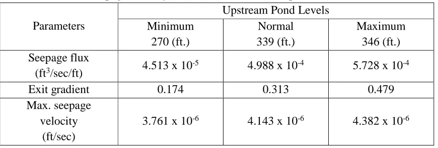
Through the study it is observed that dam safety is not endangered from the seepage point of view since the phreatic line pattern follows standard design criterion. For the three scenarios of Minimum, Normal and Maximum pool levels the exit gradient value is within permissible limits (i.e. less than 1.0). Estimated seepage flux is minimum and maximum seepage velocity is within safe limits. Fig. 4.3 - Fig. 4.6 show a graphical relationship for exit gradient and maximum seepage velocity as a function of pond level respectively. Cut off wall exhibit substantive effect on dissipating the residual head, and therefore its effectiveness and of the core wall is demonstrated significantly.
evaluate the performance of the model are found to be 2.445ft, 1.413 ft, 1.379% and 99.442% respectively. Additionally verifiability of the model is also made by comparing observed and simulated values of piezometeric heads; such graph is illustrated in Fig. 6. The slope of the line is observed to be approximately at 45 degree; thus the Fig. indicates no
considerable difference between
observed and simulated head values.
Keywords: Seepage Analysis, Phreatic Line, Earthen dam, SEEP/W, Finite Element Modeling.
INTRODUCTION
The theory of flow through porous media enables an engineer to predict the amount of water seeping through and under an earthen dam along with the water pressure distribution. It plays a pivotal role in dam engineering. Forchheimer in (1880’s) testified that the distribution of water pressure and velocity within a seepage medium obey the Laplace equation. Later in (1900’s) Forchheimer introduced a graphical method. Richardson (1920) also contributed towards solution of Laplace equation and its application in seepage analysis of earthen dam, which was further refined by supplemental research work carried out by Casagrande L. in (1937). Graphical procedures or electric models are also available techniques for studying the seepage analysis in order to devise effective measures to ensure dam
Some main factors which are responsible for contributing towards seepage are: (a) high permeability; (b) short seepage courses; (c) cranks and fissures; and (d) uneven settlement which gives rise to gaps or cracks in the soil or between soil and structure. Excessive seepage may be minimized by using low permeability soil, inserting core walls in earth structure or providing cutoff walls in foundation; upstream blankets and widening of seepage channels also help in reducing seepage quantity Khattab, (2010). Safe and secure designing of earthen dam necessitates ensuring effective and flawless seepage and sloping stability analysis Siddappa et al., (2006). The dam’s having sloping core are more efficient and viable economically, it is only due to the fact that grouting can be achieved, when the process of erecting the downstream pervious embankment is in progress www.dur.ac.uk., (2006).
saturated and unsaturated porous body of any earth fill dam Tayfur et al., (2004). The SEEP/W software of Geo-Slope Company can be put into effect for modeling and analysis of seepage Goharnejad et al. (2010).
In this research work, finite element approach is employed to solve the governing differential equations pertaining to seepage through body of dam its foundation. For this purpose, the foremost focal point is discretization of domain into finite elements by placement of imaginary nodal points and discretization of governing equations into a system of equations; an equation for each nodal point or element and solving it for the unknown variables. The SEEP/W software (program) is a sub-program of the Geo-Slope (software) computer, which is used to cater for seepage problems through porous soil media. The Geo-Slope is windows based computer software which is fully versatile to solve various types of geo-tech problems with high degree of proficiency and accuracy Geo-Slope International (2007).
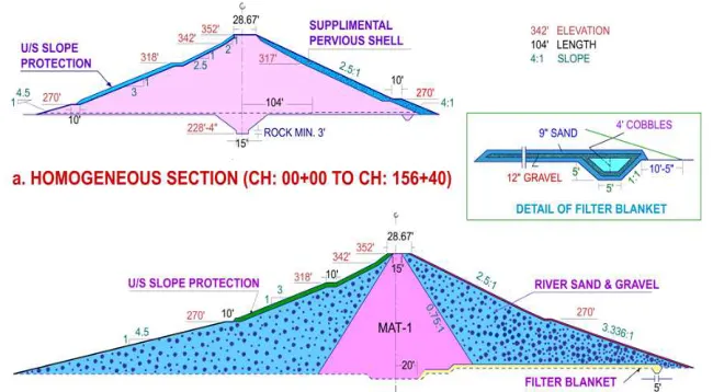
In view of all above facts, the present research work is designed to model seepage analysis of an earthen dam by using finite element approach. For this purpose a research study was conducted on Hub dam, which is a small earthen dam located at about 35 km, north-east of Karachi city, Pakistan. The main dam is 15,640 ft long and 152 ft high earthen embankment. Except for a 3,100 ft reach
(between Ch. 32 + 00 to 63+00) of non- homogeneous (zoned embankment) section in river valley, the entire length of the embankment is made of homogenous section with a supplemental downstream shell of pervious material. The zoned embankment has silt (intermixed ML and CL material) and clean river sand-gravel in shoulder of the closure section Arshad.I etal., (2014).
OBJECTIVES
The objective(s) of this research work was to study the seepage behavior of earthen dam by using Finite Element analysis, to simulate phreatic line of seepage for homogenous and non-homogeneous section for various scenarios of the dam; to develop and calibrate a computer model for an earthen dam using FEM based software i.e. the SEEP/W, and to compare observed and simulated data.
MATERIALS AND METHODS
Steps for Modeling of Hub Dam
Dirichlet and Neumann boundary nodes. The nodes at the bottom of the foundation of dam are considered with zero-flux (Nuemann) condition. After the development of complete model, it is verified by the SEEP/W software and computation for different scenarios of water levels is carried out accordingly. The material properties for the materials used in dam section are calibrated. Finally simulated results obtained from the SEEP/W software for each section are compared with the field observations obtained from the WAPDA Pakistan.
GOVERNING EQUATIONS
In this research work, finite element approach is employed to solve the governing differential equations pertaining to seepage through body of dam its foundation. The SEEP/W software (program) is a sub-program of the Geo-Slope (software) computer, which is used to cater for seepage problems through porous soil media. SEEP/W is a FEM based CAD type software used to analyze seepage and groundwater flow problems. Following partial differential equation (PDE) is the governing equation used for modeling of SEEP/W program:
…..1
Where;
H- is hydraulic head, Kx- and Ky- are hydraulic conductivity in x- and y- directions, respectively, Q- is the applied source or sink terms, t- is the time
domain and volumetric water content.
SELECTION OF CROSS SECTIONS FOR FEM MODELING
Since the main dam is composed of different kinds of reaches, therefore one cross-section from each reach i.e. Homogenous and Non-homogenous section is selected respectively.
(i) Section -I: Homogenous section at CH: 29+00.
(ii) Section-II: Non-homogenous Section (Zoned embankment section with 28.5 ft
wide cut-off wall) at CH: 56+00.
Fig. 1: Geometry of Section-I and Section-II.
FEM Mesh Formation and Its
Verification by Using SEEP/W
Software
FEM meshes for the selected sections i.e. Section- I, and -II are developed by using the SEEP/W software. The material properties for each section with proper dimensions are made as input to the software respectively and
verification for each cross section has been made accordingly.
The FEM mesh at homogenous Section-I is composed of four types of elements, i.e. triangular, square, rectangular and trapezoidal type of elements of different sizes (Fig. 2.1). The domain is discretised into a mesh by 12,346 elements through placement of nodal points 12,495.
Likewise Section-II, as displayed in Fig. 2.2, is segregated into 2,206 elements by using triangular, square, rectangular and trapezoidal type of elements through placement of 2,297 nodes.
Fig. 2.2: Mesh Formation for Zoned Embankment Section-II at Ch: 56+00.
After all the necessary inputs, the computer program SEEP/W verified the mesh development and delivered report that the vertical and horizontal meshing is strong enough and there is no error in formation of mesh models. Thus the model is ready for computation and analysis of the results.
SETTING OF BOUNDARY
CONDITIONS
Computations are carried out for following three different scenarios, viz: (i) Maximum pool level (346 ft), (ii)
Normal pool level (339 ft), and (iii) Minimum pool level (270 ft). Boundary conditions are set as: (i) At fill level up- and down-stream boundary conditions are considered as Dirichlet boundary conditions for all the above given scenarios, and (ii) In foundation up-, down- and bottom level are considered as with zero-flux condition
i.e. Neuman boundary conditions for all the above given conditions.
PROBLEM CONSIDERED FOR ANALYSIS AND COMPUTATION
The following problems are to be considered for analysis and computation:
Development of flow net by tracing streamlines and equipotential lines for different conditions.
Observation of velocity vectors and thereby seepage behaviour for different conditions.
Profile of the phreatic line for different conditions.
Estimation of seepage quantity through the dam profile and its foundation for different conditions.
head along the dam foundation under different conditions.
RESULT DISCUSSION
Calibration of Material Properties of Hub Dam Model
For calibration of material properties for the three selected sections of the Hub dam, initially identical guess values were specified for all the sections. These guess values for different types of materials used in the dam are presented below in Table 1.1. Calibration of the material properties is made on the basis of minimization of error while comparing observed hydraulic heads with the simulated ones.
Table 1.1: Material Properties (Guess Values)
S. No
Material type
* Hydraulic conductivity
(ft/sec) 01 Foundation 10-4 to 10-6
02 Shell 10-5 to 10-6
03 Core 10-8 to 10-7
04 Filter
Blanket 10
-2
* Source: WAPDA
Using SEEP/W software, the
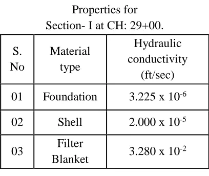
material properties (hydraulic conductivities) calibrated for all the two selected sections; viz: homogenous Section-I at CH: 29+00, non-homogenous (zoned embankment)Section-II at CH: 56+00 are presented in Table 1.2, and Table 1.3 respectively.
Table 1.2: Calibrated Values of Material Properties for
Section- I at CH: 29+00.
S. No
Material type
Hydraulic conductivity
(ft/sec)
01 Foundation 3.225 x 10⁻⁶
02 Shell 2.000 x 10⁻⁵
03 Filter
Blanket 3.280 x 10
-2
Table 1.3: Calibrated Values of Material Properties for
Section- II CH: 56+00
S. No
Material type
Hydraulic conductivity
(ft/sec)
01 Foundation 3.000 x 10⁻⁶
02 Shell 2.385 x 10⁻⁵
03 Core 2.000 x 10⁻⁸
04 Filter
Blanket 3.280 x 10
-2
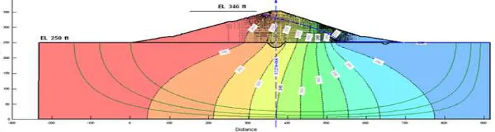
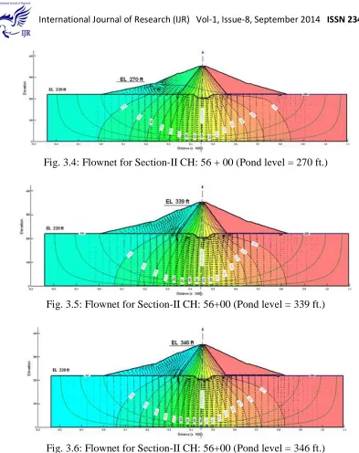
Flownet with Stream- and
The SEEP/W software is used to get seepage analysis through the dam and its foundation for different pond level scenarios. For this purpose, using the software flownet has been drawn for all the selected sections as shown in Fig. 3.1 – 3.6. The flownet comprises of streamlines, equipotential lines, velocity vectors showing dominant flow (seepage) field and phreatic line
depicting seepage behavior of the Hub dam. From the Figs. it is revealed that the stream and equipotential lines are normal to each other, which conforms to seepage theory. The effectiveness of filter blanket at higher pond levels is more significantly demonstrated at Section-I. Similarly effectiveness of core wall in Section-II is also demonstrated in the pertinent Figs.
Fig. 3.1: Flownet for Section-I CH: 29+00 (Pond level = 270 ft).
Fig. 3.2: Flownet for Section-I CH: 29+00 (Pond level = 339 ft.)
Fig. 3.4: Flownet for Section-II CH: 56 + 00 (Pond level = 270 ft.)
Fig. 3.5: Flownet for Section-II CH: 56+00 (Pond level = 339 ft.)
Fig. 3.6: Flownet for Section-II CH: 56+00 (Pond level = 346 ft.)
Seepage Flux, Exit Gradient and Maximum Seepage Velocity
Using the SEEP/W software, the seepage flux (discharge), exit gradient and maximum seepage velocity for the entire pond level scenarios and for all the selected sections are computed; these are listed in Table 1.4 and Table 1.5 accordingly. At lowest pond level
minimum seepage occurs and amongst all the sections minimum seepage occurs at section-I; that is of the order of 4.513 x 10⁻⁵ (ft3/sec/ft); at highest pond level
maximum seepage occurs and amongst all the sections maximum seepage occurs at section-II; and which is of the order of 5.798 x 10⁻⁴ (ft3/sec/ft). A
versus pond level is also shown in Fig. 4.1and 4.2 respectively. Almost for all the scenarios a linear trend is observed.
Likewise it is also ascertained that the exit gradient is within the permissible limits that is that less than unity for all the scenarios and at all the selected
sections for study; thus it also conforms to safety criteria of the dam. Fig. 4.3 and Fig. 4.4 show a graphical relationship for exit gradient as function of pond level respectively. In this case initially a linear behavior is followed; however the exit gradient rises exponentially as the pond level increases.
Table 1.4: Computed seepage flux, exit gradient and maximum seepage velocity at Section-I for different pond levels
Parameters
Upstream Pond Levels Minimum
270 (ft.)
Normal 339 (ft.)
Maximum 346 (ft.) Seepage flux
(ft3/sec/ft) 4.513 x 10
-5 4.988 x 10⁻⁴ 5.728 x 10⁻⁴
Exit gradient 0.174 0.313 0.479
Max. seepage velocity
(ft/sec)
3.761 x 10⁻⁶ 4.143 x 10⁻⁶ 4.382 x 10⁻⁶
Table 1.5: Computed seepage flux, exit gradient and maximum seepage velocity at Section-II for different pond levels
Parameters
Upstream Pond Levels Minimum
270 (ft.)
Normal 339 (ft.)
Maximum 346 (ft.) Seepage flux
(ft3/sec/ft) 2.113 x 10⁻⁴ 5.470 x 10⁻⁴ 5.798 x 10⁻⁴
Exit gradient 0.099 0.188 0.317
Max. seepage velocity
(ft/sec)
1.002 x 10⁻⁶ 2.490 x 10⁻⁶ 3.024 x 10⁻⁶
Similarly seepage velocities for the entire pond level scenarios and for all the selected sections are computed; at lowest pond level minimum seepage velocity is observed and amongst all the sections minimum velocity occurs at section-II; which is of the order of 1.002
maximum velocity occurs and amongst all the sections maximum velocity occurs at section-I; and is of the order of 4.382 x 10⁻⁶ (ft/sec). Fig. 4.5 and Fig. 4.6
velocity rises exponentially as the pond level goes up on increasing.
Fig. 4.1: Seepage flux vs. pond levels at Section-I.
Fig. 4.2: Seepage flux vs. pond levels at Section-II.
Fig. 4.3: Exit gradient vs. pond levels at Section-I.
Fig. 4.4: Exit gradient vs. pond levels at Section-II.
Fig. 4.5: Max. seepage velocity vs. pond levels at Section-I.
Fig. 4.6: Max. seepage velocity vs. pond levels at Section-II.
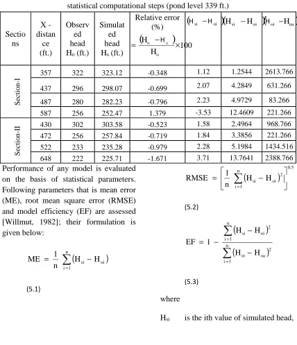
Residual Head Dissipation Trend
Residual head dissipation trend is also modeled and predicted for all the sections of interest for different scenarios; this is displayed in Fig. 5.1(a) through Fig. 5.1(c). It is revealed from these graphs that at Section-I at low pond level slightly smoother dissipation rate is followed (Fig. 5.1(a)) , however, at higher pond levels a somewhat rapid dissipation of head occurs at sheet pile positions (Fig. 5.1(b)-(c)); this of course signifies the effectiveness of sheet pile.
however at the position of core wall and sheet pile an abrupt rise in dissipation of head is exhibited, which again signifies the effectiveness of the two seepage control devices.
Fig. 5.1 (a): Head dissipation trend along the dam foundation
Section-I (270 ft. pond level)
Fig. 5.1 (b): Head dissipation trend along the dam foundation
Section-I (339 ft. pond level)
Fig. 5.1 (c): Head dissipation trend along the dam foundation
Section-I (346 ft. pond level)
Fig. 5.2 (a): Head dissipation trend along the dam foundation
Section-II (270 ft. pond level)
Fig. 5.2 (b): Head dissipation trend along the dam foundation
Section-II (339 ft. pond level)
MODEL VALIDATION
Validation of any model is made by comparing predicted results against the field observations for the acceptability of the model. If the comparison shows a good coincidence, then the model
developed can be recommended for practice. Table 1.6 contains the data pertaining to observed piezometeric heads and simulated ones and the relative error.
Table 1.6: Observed and simulated hydraulic heads with statistical computational steps (pond level 339 ft.)
Sectio ns X - distan ce (ft.) Observ ed head Ho (ft.)
Simulat ed head Hs (ft.)
Relative error (%) S ec ti o n -I
357 322 323.12 -0.348 1.12 1.2544 2613.766
437 296 298.07 -0.699 2.07 4.2849 631.266
487 280 282.23 -0.796 2.23 4.9729 83.266
587 256 252.47 1.379 -3.53 12.4609 221.266
S ec ti o n -I
I 430 302 303.58 -0.523 1.58 2.4964 968.766
472 256 257.84 -0.719 1.84 3.3856 221.266
522 233 235.28 -0.979 2.28 5.1984 1434.516
648 222 225.71 -1.671 3.71 13.7641 2388.766
Performance of any model is evaluated on the basis of statistical parameters. Following parameters that is mean error (ME), root mean square error (RMSE) and model efficiency (EF) are assessed [Willmut, 1982]; their formulation is given below:
(
)
∑
= − = n 1 i oi si H H n 1 ME (5.1)(
)
0.5n 1 i 2 oi si H H n 1 RMSE − =
∑
= (5.2)(
)
(
)
∑
∑
= = − − − = n 1 i 2 oa oi n 1 i 2 oi si H H H H 1 EF (5.3) whereHsi is the ith value of simulated head,
(
)
2 oa oi HH −
(
)
2oi
si H
H −
(
Hsi −Hoi)
(
)
100 H H H o so − ×
Hoi is the ith value of observed head,
and
Hoa is the average or mean of
observed head.
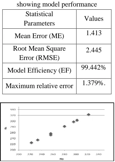
The EF is another parameter to evaluate the performance of the model. For the developed simulation model, RMSE and ME values are found 2.445 and 1.413 ft, respectively (Table 1.7) and the maximum relative error amongst all the data sets is 1.379 %. Thus it is found that the performance of the model is good enough with model efficiency of 99.442 %.
Table 1.7: Summary of statistical parameters
showing model performance Statistical
Parameters Values
Mean Error (ME) 1.413
Root Mean Square Error (RMSE)
2.445
Model Efficiency (EF) 99.442%
Maximum relative error 1.379%.
Fig. 6: Relationship between observed and simulated hydraulic heads.
Additionally verifiability of the model is also made by comparing observed and simulated values of piezometeric heads; such graph is illustrated in Fig. 6. The slope of the line is observed to be approximately at 45 degree; thus the Fig. indicates no considerable difference between observed and simulated head values. Consequently, it is concluded that simulated values of piezometeric heads are not much different than the observed ones.
CONCLUSIONS
In the present study a computer model for Hub dam based on FEM using SEEP/W software has been developed and calibrated. The model has been used to study the seepage behavior of the hub dam for two different sections i.e. section –I (Homogenous) and Section – II (Non-Homogeneous), for three different scenarios of Minimum, Normal and Maximum pool levels i.e. 270, 339 and 346 ft, respectively. The phreatic line has been simulated at each section for the three scenarios and compared with field observations and the model demonstrates high efficiency and good fitness.
permissible limits (i.e. less than 1.0) for both sections, which implies that the dam is safe against piping for all the scenarios and there is no any possibility of internal erosion due to seepage. Estimated seepage flux is minimum and maximum seepage velocity is within safe limits.
Fig. 4.3 - Fig. 4.6 show a graphical relationship for exit gradient and maximum seepage velocity as function of pond level respectively. Under this case at first a linear behavior is followed, however the velocity rises exponentially as the pond level goes up on increasing. This is because initially there was a linear laminar flow but as the pond level is rising the flow is laminar but non-linear.
Cut off wall exhibit substantive effect on dissipating the residual head, and therefore its effectiveness and of the core wall is demonstrated significantly. For the case of Hub dam, it is found that construction of impervious cut-off wall at Section-II has a small effect on decreasing the quantity of seepage; this is because the imperviousness of foundation material is dominant over shell material.
Statistical analysis of all the research data i.e. RMSE, ME, R.E, and EF to evaluate the performance of the model are found to be 2.445ft, 1.413 ft, 1.379% and 99.442% respectively. Additionally verifiability of the model is also made by
comparing observed and simulated values of piezometeric heads; such graph is illustrated in Fig. 6. The slope of the line is observed to be approximately at 45 degree; thus the Fig. indicates no considerable difference between observed and simulated head values. Consequently, it is concluded that simulated values of piezometeric heads are not much different than the observed.
SUGGESTIONS
This research study suggests that Geo-Slope SEEP/W software requires that the user to be proficient in dam design concepts. This software can help the water resource engineer to use it in testing and analyzing any alternative design hydraulically and economically. Due to transient characteristic of this software, it provides a window of opportunity for researchers to analyze such problems; for instance migration of a wetting front and dissipation of excessive pore water pressures.
ACKNOWLEDGEMENTS
REFERENCES
[1] I. Arshad and M.M. Baber (2014)
“Comparison of SEEP/W
Simulations with Field Observations for Seepage Analysis through an Earthen Dam (Case Study: Hub Dam - Pakistan)”. Published in International Journal of Research (IJR), Vol-1, Issue-7, August 2014. ISSN: 2348-6848.
[2] H. Gohanejad, M.Noury, A. Noorzad, A. Shamsaie (2010), “The Effect of Clay Blanket Thickness to Prevent Seepage in Dam Reservoir”. Research journal of Environmental Sciences, ISSN 1819 – 3412. [3] S. A. A. Khattab (2010)
“Stability Analysis of Mosul Dam under Saturated and Unsaturated Soil Conditions”. Al- Rafidain Engineering Journal Vol. 18 No. 01.
[4] Gopi Siddappa, K. S. Hariprasad, I. A. Abdul Hussain (2006), “Transient Seepage Analysis of an Earth Dam: Sensitivity to Anisotropy and Soil Properties”. Journal of Water Power Magazine Volume XVI, Issue 4. [5] T. K. Hnang (1999) “Stability
Analysis of an Earth Dam Under Steady State Seepage” Online University Journal, Department of Civil Engineering, Chung- Hsing University, Taichung 40227, Taiwan.
[6] Terzaghi, K., Peck, R. B., and Mesri, (1996), "Soil Mechanics in Engineering Practice", 3rd edition, Wiley, New York. [7] WAPDA, (2009), “4th Periodic
Inspection Report of Hub Dam”, ACE – WAPDA.
[8] Williams, E., (1986), "Seepage Analysis and Control for Dams", Department of the Army U.S. Army Corps of Engineers, Washington.
[9] Geo-Slope Software Example (2007),” Seepage through A Dam
Embankment”. Geo-Slope