Volume 2007, Article ID 51684,10pages doi:10.1155/2007/51684
Research Article
Pushing it to the Limit: Adaptation with Dynamically
Switching Gain Control
Matthias S. Keil1and Jordi Vitri `a1, 2
1Centre de Visi`o per Computador, Edifici O, Campus UAB, 08193 Bellaterra, Cerdanyola, Barcelona, Spain
2Computer Science Department, Universitat Aut`onoma de Barcelona, 08193 Bellaterra, Cerdanyola, Barcelona, Spain
Received 1 December 2005; Revised 11 July 2006; Accepted 26 August 2006
Recommended by Maria Concetta Morrone
With this paper we propose a model to simulate the functional aspects of light adaptation in retinal photoreceptors. Our model, however, does not link specific stages to the detailed molecular processes which are thought to mediate adaptation in real photore-ceptors. We rather model the photoreceptor as a self-adjusting integration device, which adds up properly amplified luminance signals. The integration process and the amplification obey a switching behavior that acts to shut down locally the integration process in dependence on the internal state of the receptor. The mathematical structure of our model is quite simple, and its com-putational complexity is quite low. We present results of computer simulations which demonstrate that our model adapts properly to at least four orders of input magnitude.
Copyright © 2007 M. S. Keil and J. Vitri`a. This is an open access article distributed under the Creative Commons Attribution License, which permits unrestricted use, distribution, and reproduction in any medium, provided the original work is properly cited.
1. INTRODUCTION
There is agreement that adaptation (i.e., the adjustment of sensitivity) is important for the function of nervous systems, since without corresponding mechanisms, any neuron with its limited dynamic range would stay silent or operate in sat-uration most of the time [1]. Because neurons are noisy de-vices, reliable information transmission is only granted if the distribution of levels in the stimulus matches the neuron’s reliable operation range [2].
Consider, for example, the mammalian visual system, with the retina at its front end. When performing sac-cades, the retina must cope with intensity variations which may span about one [3, 4] to about two orders of mag-nitude (2 including shadows according to [3], 2-3 accord-ing to [5]). From one scene to another (e.g., from bright sunlight to starlight), the range of intensity variations may well span up to ten orders of magnitude [6–9]. This range of intensities has to be mapped onto less than two orders of output activity of retinal ganglion cells [10], implying some form of compression of the scale of intensity val-ues. The retina achieves this by making use of a cascade of gain control and adaptation mechanisms, respectively (e.g., [11–14]). Specifically, cone photoreceptors may decrease their sensitivity proportionally to background intensity, over
about 8 log units of background intensity [15]. This relation-ship is known as Weber’s law (e.g., [16]). Adaptation in pho-toreceptors is achieved by subtly balanced network of molec-ular processes (see [17] for an excellent introduction, and [14,18] with references). Many of the data were gained from rod photoreceptors because they are more amenable to anal-ysis. It is generally believed, however, that similar processes are also taking place in cones.
defined by low contrasts, whereas no activity exchange oc-curs between regions which are separated by high contrast boundaries (very similar to an anisotropic diffusion mech-anism [25]). In this way, contrast adaption is implemented. Notice that our model lacks the latter stage, and only simu-lates the photoreceptor adaptation.
2. MECHANISMS OF ADAPTATION IN THE RETINA
A response to light is initiated by photoisomerization of the chromophore 11-cis-retinal to all-trans-retinal. In dark-ness, 11-cis-retinal is bound to rhodopsin in its inactive conformation, and lies buried in the membranes of the outer segment discs. Upon absorption of a photon, and the subsequent photoisomerization of the chromophore, the rhodopsin undergoes a conformational change which con-verts it into its active form Rh∗ (or metarhodopsin II). The presence of Rh∗ triggers two distinct mechanisms: a recy-cling process known as visual cycle, and an enzymatic cas-cade known as transduction cascas-cade.
The visual cycle begins with the phosphorylation of Rh∗, and subsequent binding of arrestin to the phosphorylated photopigment. After, binding of arrestin, the photopigment is rendered completely inactive. The protein opsin is then de-phosphorylated, and retinal is reduced to all-trans-retinol. The retinol is isomerized to the 11-cis-isomer outside the photoreceptor (in the adjacent retinal pigment epithe-lium layer), and reenters afterwards to recombine with the dephosphorylated opsin.
The transduction cascade begins with the serial activa-tion of transducins by Rh∗, implementing the first stage for signal amplification in the cascade [26]. Thereby, an active complex Tα·GTP is formed, which binds to and activates the enzyme phosphodiesterase (PDE). PDE reduces the concen-tration of cytoplasmatic cGMP by hydrolizing it. The latter process constitutes a second stage for amplification. The hy-drolysis of cGMP causes the closing of cGMP-gated channels, what in turn generates the electrical response of photorecep-tors. Thus, photoreceptors are depolarized in darkness be-cause of their open cationic channels, and get hyperpolarized by light. In darkness, the steady current that flows into the outer segment is usually called dark or circulating current.1
The main fraction of the circulating current is carried by Na+ ions, and a smaller fraction of Ca2+ions [27]. Calcium
is transported out of the outer segment by the Na+/K+-Ca2+
-exchange protein at a constant rate, independent of the light hitting the photoreceptor. This implies that light decreases intracellular Ca2+levels, because of the increased probability
of channel opening. As a consequence, a direct correlation (i.e., a linear relationship) exists between the circulating cur-rent and Ca2+concentration.
Adaptation of the photoreceptor to ambient light is granted by balancing the just described amplification mech-anisms (for low light situations) against mechmech-anisms which
1The photocurrent is brought back to the dark-adapted level by hydrolizing the GTP to GDP.
Table1:Model overview: an overview over the mechanisms used in the model of Grossberg and Hong [19,20] and our approach.
Mechanism [19,20] Our approach
Light adaptation Yes Yes
Local divisive gain control No Yes
prevent response saturation (e.g., for sunlit scenes). This bal-ance is implemented by feedback mechanisms which act ei-ther on the catalytic activity or on the catalytic lifetime of the components that make up the phototransduction cascade [28]. It is now well established that changes in Ca2+
concen-tration regulate the cascade in at least three important ways. First, Ca2+ can prolong the lifetime of Rh∗through the
inhibition of phosphorylation in the visual cycle, by means of recoverin. Second, in the transduction cascade, Ca2+
reg-ulates the cytoplasmatic concentration of cGMP by bind-ing to guanylate cyclase—the enzyme that is responsible for cGMP synthesis. Third, decreasing Ca2+ concentrations
in-creases the sensitivity of the cationic channels to cGMP [29]. Taken together, Ca2+ is now considered as the
photore-ceptor’s internal messenger for adaptation. Supporting evi-dence comes from the fact that adaptation effects can be pro-voked without light (cf. [14, page 130]), by only lowering the Ca2+ concentration, or that adaptation is suspended by
clamping the Ca2+ level to its value corresponding to
dark-ness (see [14, page 126]).
Beyond the level of the individual photoreceptor, fur-ther mechanisms related to adaptation are effective, for ex-ample network adaptation in interneurons and retinal gan-glion cells (i.e., adaptation is “transferred” beyond the recep-tive field of the actually stimulated cell, e.g., [30–33]), and discounting predictable spatio-temporal structures from the stimulus by Hebbian mechanisms [34,35].
3. FORMAL DEFINITION OF THE ADAPTATION DYNAMICS
Table 1gives a brief comparison of components, and a sketch of our model is shown in Figure 1. In what follows, we give the formal introduction to our mechanisms which are thought to provide an abstract view for adaptation as it takes place in the outer segment of individual photoreceptors.
Let Li j be a two-dimensional luminance distribution which provides the input into our model. For the purpose of the present paper, we assume that the model converges before changes in luminance occur, that is,∂Li j(t)/∂t = 0, where spatial coordinates are denoted by (i,j). We assume that the input is normalized according to <L ≤1, with
is chosen such that 0<<mini,j{Li j}. LetPdenote the membrane potential of the photoreceptor, which is assumed to obey the equation (the symbolsgleak,gexc(t), andVexcare
defined below)
dP(t)
dt = −gleakP(t) +gexc(t)
Vexc−P(t)
Luminance
Gain control #1 S(t)
Gain control #2 G(t),Θ(t)
F
eedbac
k
F
eedbac
k
Gating
Photoreceptor membrane potentialP
Output
Figure1:Model sketch: a luminance distribution is subjected to a divisive “gain control” stage #1 (S(t), (3)). At this stage, inhibition of luminanceLtakes place as a function of increasing photorecep-tor potentialP. The second gain control stageG(t) can either am-plify the signalS(t) or attenuate it ((4), (5), and (6)). Amplification ofS(t) occurs if the membrane potentialPfalls below a threshold
Θ, and attenuation forP >Θ(see (5)). Both “gain control” stages interact multiplicatively (denoted by the symbol “⊗,” (2)) before providing excitatory input into the photoreceptor’s membrane po-tential (symbol “P,” (1)). The photoreceptor potential in turn feeds back into both of the “gain control” stages. At the same time, the photoreceptor potential represents the output of our model.
Table2:Simulation details: the table is self-explanatory. For the in-tegration of (1), a fourth-order Runge-Kutta scheme was used with an integration time step of 0.01. The remaining differential equa-tions were integrated with Euler’s method with an integration time step of one. Notice that the integration step sizes were not adjusted to match physiological time scales.
Parameter Value Equation Description
gleak 0.05 (1) Leakage conductance
Vexc 1 (1) Synaptic battery
γ 1.5 (3) Divisive gain
τ1 0.7213 (5) Damping time constant
τ2 −40.4979 (5) Amplification time constant
Θ0 0.25 (6) Initial threshold value
τΘ 39.4949 (6) Threshold decay time constant
An instance of the last equation holds for each position (i,j), henceP ≡Pi j(t) (in what follows, indices were dropped for brevity). The excitatory saturation point (or reversal poten-tial) is defined byVexc, and the leakage (or passive)
conduc-tance is defined bygleak(note thatVexcrepresents an
asymp-tote forP). Both of the last constants are equal for all pho-toreceptor cells. The default simulation parameters, as well as further simulation details, can be found inTable 2. No-tice that photoreceptors in fact hyperpolarize in response to light (cf.Section 2), whereas the last equation makes a con-trary assumption. This assumption, however, implies no loss of generality, since the model can equivalently be reformu-lated such that it hyperpolarizes with increasing intensity levels.
Luminance 256256 pixels (a)
γ=1.5 (default) (b)
γ=0 (no divisive gain) (c)
Figure 2:Artifacts with a luminance ramp.(a) The inputLi j, a luminance step with a superimposed luminance ramp (increasing linearly from left to the right). (b) With the default valueγ =1.5 in (3), the adaptated image is correctly rendered and hardly distin-guishable from the input. (c) Settingγ =0 causes the appearance of ripple artifacts in the adaptated image. All results are shown at t=250 iterations.
Excitatory input to the photoreceptor potential is given by the conductancegexc≡gexc,i j(t), which is defined by
gexc(t)=G(t)·S(t), (2)
where the processG ≡Gi j(t) interacts multiplicatively with the light-induced signal S ≡ Si j(t) (such interaction was previously referred to as mass action or gating mechanism, see [21]). For the signalS, we assume that its efficiency for driving the photoreceptor’s potential diminishes with in-creasing potentialP:
S(t)= L
1 +γ·P(t). (3)
The last equation in fact establishes a feedback mechanism which allows the photoreceptor to regulate the strength of its own excitatory input. In addition, the excitatory drive of the photoreceptor is also a decreasing function of increasing po-tentialP(t) by virtue of the term “(Vexc−P)” (the driving
potential) in (1). Notice that ifgexc was constant and suffi
-ciently high, the driving potential would makeP(t) saturate at Vexc (i.e.,Vexc is asymptotically approached). Therefore,
both the excitatory inputgexc and the driving potential
de-crease asP(t) grows. The motivation for including (3) in our model was to eliminate ripple artifacts seen with luminance ramps (Figure 2). With “normal” natural images, those arti-facts did not appear to be a major nuisance (Figure 3, see also
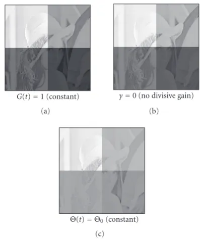
G(t)=1 (constant) (a)
γ=0 (no divisive gain) (b)
Θ(t)=Θ0(constant) (c)
Figure3:Artifacts: the results shown in this figure should be com-pared withFigure 7. (a) Setting the amplification constant toG(t)= 1 in (2) diminishes adaptation (i.e., low luminance values are not pushed that high). Notice that in this case dynamical switching is made inoperative. (b) Settingγ=0 in (3) has no effect on the nat-uralimages we have tested, but causes strong ripple artifacts with luminance ramps as demonstrated inFigure 2. (c) Using a constant thresholdΘ(t) =Θ0 =0.25 in (5) leads to strong saturation (or
over-adaptation). All results are shown att=250 iterations.
The processG(t) implements an amplification mecha-nism as follows:
τkdG(t)
dt = −G, (4)
where the initial conditionG(t = t0) =1 was used.
Simu-lations are assumed to start att0 = 0. By virtue of the
in-dexk ∈ {1, 2}associated with the time constantτk, the last equation describestwodistinct processes. These processes are characterized by τ1 > 0 (making G decay with time), and
τ2 < 0 (leading to an increase of G with time). The last
equation thus implements what we dubbed a “dynamically switching gain control.” But who or what is switchingGon (i.e., making it increase with|τ2|) or off(i.e., making it
de-crease withτ1)? The one or the other process is invoked
de-pending on whetherPexceeds a thresholdΘor not:
k=1 ifP(t)>Θ(t),
k=2 otherwise. (5)
This means that if the outer segment potentialPis below the thresholdΘ, its inputgexc(t) is amplified via (3). The
ampli-fication mechanism acts to diminish the integration time of luminance signals until reaching the thresholdΘ, especially low-intensity signals. Once the threshold is exceeded, ampli-fication is switched off(Figure 5). In fact,G decays rapidly
then in order to avoid driving the outer segment potential into saturation (which nevertheless may occur at sufficiently high intensity values). With ineffective dynamical switching G ≡const adaptation is severely deteriorated (Figure 3(a)). Mathematically, the dynamic switching mechanism avoids an unbounded growth ofG.
Amplification proceeds untilP crosses a threshold. The threshold, however, is not fixed, but is rather represented by a slowly decaying process on its own:
τΘdΘdt(t)= −Θ(t). (6)
We used the initial conditionΘ(t = t0) = Θ0, and like to
point out that the thresholdΘis not supposed to represent a firing threshold for the photoreceptor. It rather serves to implement the dynamic switching behavior for turning the signal amplification on or off. The motivation for includ-ing a dynamical threshold in our model was the elimina-tion of artifactual contrasts inversion effects, and will be ex-plained in more details inSection 4. Furthermore, if a con-stant threshold was chosen, over-adaptation would occur (Figure 3(c)).
Our simulations were evaluated at the moment when Pi j > Θi j for all (i,j). This is, however, not a steady state, because the outer segment potential continues to decay with gleak. The results which are presented in Figures8to10
there-fore show snapshots of the outer segment potential at exactly the moment when the last potential valuePi j(t) exceeded the thresholdΘ(t) (i.e., (i,j) corresponds to the position with the lowest intensity value in the input).
One may ask why we gave preference to a dynamical for-mulation of our model over steady state equations. Intu-itively, steady state solutions cannot capture the full behavior revealed by the model. For example, the steady state solution (as defined bydΘ/dt =0) of the last equation is zero, and, depending on k, the steady state solution of (4) is infinity (k=2) or zero (k=1).
4. DESCRIPTION OF THE ADAPTATION DYNAMICS
What does the adaptation dynamics defined by (1) to (6) look like? The process obviously integrates the activity gen-erated by an input image L, via the photoreceptor mem-brane potentialP. The integration proceeds untilP exceeds the threshold Θ. At this point, the integration process de-celerates exponentially with a time constant τ1 > 0, since
the corresponding solution to (4) isΘ(t)=exp(−t/τ1). The
0 1 2 3 4 5 0.5
1 1.5 2 2.5
0 0.03 0.06 0.1 0.13
log10intensity
Ti
m
e
(
t
)
PotentialP(t)
Increase in integration time
M
inim
um
int
eg
ra
tion
time
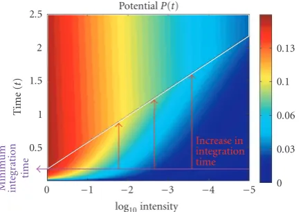
Figure4:Photoreceptor potential: the photoreceptor potentialP(1) is plotted as a function of time (t =0 to 250 iterations) and in-put intensity (L ∈ {100, 10−1,. . ., 10−5}. The photoreceptor
am-plitude is color-coded (colorbar). “Convergence” occurs when the photoreceptor potentialPexceeds a thresholdΘ, and corresponds to the area over the diagonal line. The minimum integration time is delinated by the horizontal line at the bottom. With decreasing luminance, one observes an increase in integration time until “con-vergence” is reached (as illustrated by the red arrows pointing to the plateau). A similar increase in integration time with decreasing stimulus intensity levels is also known from the retina, and is ex-pressed as Bloch’s law of temporal integration. Bloch’s law relates the threshold for seeing a stimulus to stimulus duration (i.e., inte-gration time) and stimulus intensity: the product of stimulus dura-tion and stimulus intensity equals a constant within a so-called crit-ical time window. Bloch’s law is especially prominent for scotopic vision.
plausibility. But as long as > 0, or dynamically varying noise is present in the model, eventually all luminance val-ues reach threshold in finite time, and as a consequence,G (4) switches from amplification to attenuation. This is to say that for k = 2, the process G is bounded mathematically from above. Furthermore, numerical experiments demon-strate that G does not adopt excessively high values (see
Figure 5).2
Nevertheless, a suitably parameterized and asymptot-ically bounded process for substituting G, rather than a sharply cut exponential (as it is implemented by (4), (5), and (6)), would perhaps better reflect physiological reality—but for the moment we set aside plausible functions to keep the model concise.
Why should the threshold Θdrop with time? Imagine that we fixΘ to some constant value. In that case, all lu-minance values are integrated until they all reach thesame threshold. This means that the integration process would es-tablish a common level for bright and dark luminance values, what in the best of all cases would lead to a strong reduction of contrasts with respect to the input (Figure 3(c)). But there is yet another, more technical point, to this.
2IfP(t)≤Θ(t), the subthreshold gain obeysG(t)=exp(t/|τ
2|). Assuming t=250 iterations and using|τ2| =40.5 (seeTable 2) we getG(t=250)≈ 479.55 as maximum amplification.
0 1 2 3 4 5
0.5 1 1.5 2 2.5
15 10 5 0
log10intensity
Ti
m
e
(
t
)
GainG(t)
Figure5:Dynamics of the “switching” gain control: the same as in Figure 4, but here the dynamics of the signal amplification variable G(t,L) (4) is visualized. The bright (dark) area on the bottom (top) indicates where the gain control is switched on (off). Notice that the switching occurs rather fast around the red area. The switching area resembles a blurred line—compare it to the diagonal line delineat-ing the convergence plateau inFigure 4.
Consider a pair of luminance values, one brighter than the other. Since the integration process proceeds with fixed time steps (and exponentially increasing gain), we may choose both luminance values such that they exceed the fixed threshold in a way that the previously dark luminance value leaves more super-threshold activity than the bright value (the brighter value must have exceeded threshold at some former time step, and thus its activityPalready has decayed somewhat due to the passive leakage conductance gleak in
(1)). In other words, when decoding the photoreceptor po-tentialP, the dark value would suddenly appear brighter than the original bright value. Such “contrast inversion” artifacts are avoided with a threshold that decreases with time. Thus, the dynamic threshold process (6) acts to preserve contrast polarities (notice that the threshold process asymptotically approaches zero).
Yet another type of artifact may emerge as a consequence of the exponentially increasing amplification signalG, most likely due to amplification of numerical noise while inte-grating the differential equations. With certain luminance distributions, especially with luminance ramps, step-like or ripple-like structures may appear when P is read out (of course the ripples are absent from the input, cf.Figure 2). Those artifacts are counteracted by the additional gain con-trol mechanism (3). Its net effect is to continuously decrease the integration step size for (1) as the potentialPgrows. This effect gets especially prominent for high luminance values (seeFigure 6).
5. RESULTS OF NUMERICAL EXPERIMENTS
0 1 2 3 4 5 0.5
1 1.5 2 2.5
15 10 5 0
log10intensity
Ti
m
e
(
t
)
Input signalS(t)
Figure6:Input signal: the same as inFigure 4, but here the dynam-ics of the input signalS(t,L) is visualized (3).
images with a high dynamic range could be visualized with a normal computer monitor. If we tried a direct visualiza-tion of a high dynamic range image without applying any adaptation, we could just see the luminance patterns of the first one or two orders of magnitude, while all smaller lumi-nance values would be displayed in black (seeFigure 7; notice that the optic nerve has a similar transmission bandwidth). Additionally, a “good” adaptation mechanism should leave an input image unchanged which does only vary over one or two orders of magnitude. Or at least leave such an image unchanged as far as possible. Contrast strength should ide-ally be preserved. Put another way, compression effects that are introduced by the adaptation mechanism should be min-imized.
We compare the results of our mechanism with one pro-posed in [19,20] (subsequently denoted by “Grossberg and Hong”).3
In order to assure that, at some time,P(t)i j > Θ(t) at all positions (i,j), zero values of the original luminance dis-tribution were substituted by the half of the second smallest luminance value, that is, =0.5∗min{Li j : Li j > 0}, if not otherwise stated. We used standard benchmark images of size 256×256 pixels as inputsL.
Figure 8shows the results with the MIT image, where the result obtained with our method is slightly less saturated than the one obtained with Grossberg and Hong’s method.
In order to better explore the performance of the two methods, we superimposed the original test images with arti-ficially generated illumination patterns. InFigure 9, the MIT image was multiplied with a luminance ramp to simulate an illumination gradient. In the latter case, the result from Grossberg and Hong is less saturated than ours.
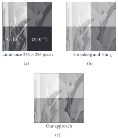
InFigure 7, the original image (shown inFigure 11) was subdivided in four “tiles,” where within each tile luminance values vary over a different order of magnitude. This test
3We implemented [20, equations (A3) to (A8)], and integrated their model over 500 iterations with Euler’s method, where a integration step size of 0.01 was used.
Luminance 256256 pixels
O(10 2) O(10 3)
(a)
Grossberg and Hong (b)
Our approach (c)
Figure7:Tiled Lena image: the original Lena image (with lumi-nance values between 0 and 1, seeFigure 11) was subdivided into four tiles, and tiles were multiplied with 100, 10−1, 10−2, and 10−3,
respectively. In the input (a), both of the lower tiles are displayed in black. The order of magnitude of the corresponding luminance range is indicated with the black tiles.
Luminance 256256 pixels (a)
Grossberg and Hong (b)
Our approach (c)
Luminance 256256 pixels (a)
Grossberg and Hong (b)
Our approach (c)
Figure 9:MIT image with overlying luminance ramp: the origi-nal MIT image (see Figure 8) was multiplied with a luminance ramp which linearly increases from left (intensity 0) to the right (intensity 1).
image mimics a situation where the range of luminance val-ues within a scene varies over four orders of magnitude. Both methods push luminance values sufficiently high such that details in the darkest tile are rendered visible (where our method yields an overall more brighter result—and hence the darkest patch is better visible). Thus, four orders of mag-nitude of input range are mapped onto two orders of magni-tude available for visualization, a situation that is similar to situations which are met by the retina.
In the last example, we created an artificial high dynamic range image (Figure 10) from the original “Peppers” im-age (Figure 11). In this case, our method produces a slightly brighter result compared with Grossberg and Hong: the re-sult generated with Grossberg and Hong’s method has harder contrasts.
We conducted further simulations where we setLi j←Pi j after convergence, and restarted the simulation. The results did not change, indicating that the model’s state after con-verging the first time already corresponds to a steady state solution.
6. MODEL BEHAVIOR WITH PARAMETER CHANGES
The parameters of our model can be tuned according to the expected numerical range of luminance values. In this way, compression effects in the output are reduced, which can lead to the generation of visually more pleasing results.
Increasing the value ofγ(Table 2; (3)) reduces the overall compression of the input at the cost of low-intensity regions. This is to say that low-intensity regions will appear darker, and regions with higher intensities will be rendered with
Luminance 256256 pixels (a)
Grossberg and Hong (b)
Our approach (c)
Figure10:Power-law-stretched Peppers image: luminance values of the original Peppers image (seeFigure 11) were raised to the power of 4 to create a high dynamic range image.
(a) (b)
Figure11:Original “Lena” and “Peppers” image: these images are shown for comparing them with the results presented in Figures7 and10, respectively.
somewhat improved contrasts. A similar effect results, albeit more intense, when increasing the threshold decay time con-stantτΘ(6). Decreasing the initial threshold valueΘ0(6) will slightly increase overall brightness and compression, respec-tively. The model behavior is quite robust against changes in the damping time constant τ1, since this mechanism is
backed up by the signal gain control stage (3). Nevertheless, variations in the value of the amplification time constantτ2
bear strongly on the results: a decrease improves greatly the adaptation behavior, but ifτ2is set too low artifacts may
oc-cur, such as contrast polarities being reversed with respect to the input. On the other hand, ifτ2 → ∞, no adaptation at
7. THIS THING CALLED “EPSILON”
As it turned out, a “smart” choice ofcan even improve the contrasts in the visualization of the results. Because for dis-playing, each image is normalized to occupy the full range of available gray levels, ifis too small with respect to the sec-ond smallest luminance value, it gets not sufficiently pushed by the adaptation process, such that in the adapted image the difference between the smallest and the second small-est value is too big. As a consequence, many of the darker gray levels are not used (if we assume a linear mapping of activity to gray levels), what leaves less gray levels for dis-playing the other (higher) luminance values. Hence, the con-trasts in the displayed image will be reduced. Ideally,should depend in some way on how dark the input image is per-ceived by a human observer. Finding an adequate function that automatically sets the value ofwould be an interesting topic for future research.
8. DISCUSSION AND CONCLUSIONS
We presented a novel theory about the adaptational mecha-nisms in retinal photoreceptors. Our theory is abstract in the sense that we did not attempt to identify model stages with components of the phototransduction cascade (as outlined in Section 2). Nevertheless, one is tempted to draw cor-responding parallels between our model and physiological data. In the transduction cascade, there are (at least) two sites of amplification: the serial activation of transducins by the active form of rhodopsin Rh∗, and the hydrolysis of cGMP by phosphodiesterase. An amplification of the sig-nal takes also place in our model by virtue of G in (4). Furthermore, Ca2+ constitutes a messenger for adaptation.
In contrast, there is no corresponding variable for describ-ing the concentration of Ca2+ in our model. Nevertheless,
the membrane potentialPsubserves two different purposes. First, it corresponds to the output of the photoreceptor. Sec-ond, it constitutes a feedback signal that acts to control signal amplification—and hence the adaptation process. As Ca2+is
known to be linearly related to the membrane potential, it seems reasonable to considerPas a lumped-together descrip-tion for both the membrane potential and the Ca2+
concen-tration.
Indeed, one can draw further parallels. In our model, sig-nal amplification stops as soon as the membrane potential exceeds a threshold, in order to counteract saturation effects (5). This process is reminiscent on the binding of arrestin to phosphorylated Rh∗, leading to a complete inactivation of the photopigment, and thus to a ceasing of the transduction cascade.
In our model, there is yet another way to counteract sat-uration effects, by means of the divisive inhibition stage (3). This process can be compared to the interaction of Ca2+with
the visual cycle, which causes an acceleration of the rate of Rh∗ phosphorylation [36–38]. This interaction is brought about by the Ca2+-binding protein recoverin, and decreases
the lifetime of Rh∗. As a consequence, less cGMP will be hy-drolyzed upon absorption of a photon [26].
On the technical side, computer simulations demon-strated that our approach is on a par with a recently proposed model by Grossberg and Hong [19,20] “(G&H).” However, several crucial differences exist between their approach and ours.
First and above all, the critical stage for adaptation in Grossberg and Hong’s approach consists of the feedback pro-vided by electrically coupled horizontal cells. Light adapta-tion through the outer segment can be decoupled from the actual adaptation dynamics, and hence may be considered as a preprocessing step in their model.
Remarkably, our approach achieves similar adaptation results without incorporating the horizontal-to-cone feed-back loop. This prediction is consistent with physiological data, as cone photoreceptors can decrease their sensitivity over about 8 log units of background intensity [15]. More-over, feedback from horizontal cells may even further im-prove adaptation. Since we have seen, on the other hand, that contrasts are reduced as a consequence of the dynamic range compression, one may speculate that feedback from hori-zontal may also compensate for this effect, by reenhancing contrasts. Notice that contrast enhancement is tantamount to center-surround interactions. Because adjacent horizon-tal cells of the same type are fused by gap junctions, their feedback will influence the membrane potential of neigh-boring cones within some radius of the actually stimulated photoreceptor. In this way, the antagonistic receptive field structure is created in bipolar cells. But then bipolar cells represent a contrast-enhanced signal of the photoreceptors. Therefore, neurophysiological data are consistent with our ideas.
Both models have similar complex with respect to pa-rameter spaces. Grossberg and Hong’s approach has some 10 parameters, whereas ours has 7 (plus the). Although we did not carry out a detailed analysis of computational complex-ity, the respective model structures suggest that the Gross-berg and Hong model is computationally more demanding. The latter fact seemed to be confirmed with our simulations on a serial computer, where our model converged in a frac-tion of the time that was necessary to achieve comparable results with the Grossberg and Hong model.4
Similar to the Grossberg and Hong model, another approach [39] is also motivated by the observation that strong contrasts usually indicate reflectance changes in nat-ural scenes, as opposed to intensity variantions due to changes in illumination. The approach in [39], however, has no stage for luminance adaptation, and only computes an “anisotropically like” smoothed version of the image, which is used for exerting divisive gain control directly on inten-sity values (cf.Table 1). The lateral connectivity between cells that form the diffusion layer is controlled by inverse We-ber contrasts. Hence, both strong and weak contrasts in the original image may affect the degree of smoothing. Simula-tion results obtained with our implementaSimula-tion of Gross’ and
Brajovic’s approach revealed strong boundary enhancement if tuned such that the adaptation was comparable to the other two methods. This suggests that the signal transduction char-acteristics of Gross’ and Brajovic’s approach are high-pass.
Our model, perhaps with different parameter values, should as well be useful for displaying high dynamic range images, or synthetic aperture radar images. This is a topic that will be pursued with future research. Further interesting questions address the incorporation of feedback from hori-zontal cells, and possibly of reset mechanisms for the thresh-old process, in order to extend our model’s processing capac-ities to image sequences.
ACKNOWLEDGMENTS
The first author M. S. Keil was supported by the Juan de la Ciervaprogram of the Spanish government. The authors acknowledge the help of two anonymous reviewers, whose comments contributed to improve the first draft of this manuscript. Further support was provided by the MCyT Grant TIC2003-00654.
REFERENCES
[1] J. Walraven, C. Enroth-Cugell, D. Hood, D. MacLeod, and J. Schnapf, “The control of visual sensitivity: receptoral and postreceptoral processes,” inThe Neurophysiological Founda-tions of Visual Perception, L. Spillman and J. Werner, Eds., pp. 53–101, Academic Press, New York, NY, USA, 1990.
[2] H. Barlow and W. Levick, “Threshold setting by the surround of cat retinal ganglion cells,”Journal of Physiology, London, B, vol. 212, p. 1, 1976.
[3] D. Hood and M. Finkelstein, “Sensitivity to light,” in Hand-book of Perception and Visual Performance, Volume 1: Sensory Processes and Perception, K. Boff, L. Kaufman, and J. Thomas,
Eds., chapter 5, pp. 5.1–5.66, John Wiley & Sons, New York, NY, USA, 1986.
[4] V. Mante, R. A. Frazor, V. Bonin, W. S. Geisler, and M. Caran-dini, “Independence of luminance and contrast in natural scenes and in the early visual system,” Nature Neuroscience, vol. 8, no. 12, pp. 1690–1697, 2005.
[5] J. H. van Hateren, “Processing of natural time series of in-tensities by the visual system of the blowfly,”Vision Research, vol. 37, no. 23, pp. 3407–3416, 1997.
[6] G. Martin, “Schematic eye models in vertebrates,”Progress in Sensory Physiology, vol. 4, p. 44, 1983.
[7] R. Shapley and C. Enroth-Cugell, “Visual adaptation and reti-nal gain controls,”Progress in Retinal Research, vol. 3, pp. 263– 346, 1984.
[8] S. B. Laughlin, “The role of sensory adaptation in the retina,”
Journal of Experimental Biology, vol. 146, pp. 39–62, 1989. [9] R. Normann, I. Perlman, and P. Hallet, “Cone photoreceptor
physiology and cone contributions to colour vision,” inVision and Visual Dysfunction, The Perception of Colour, P. Gouras, Ed., pp. 146–162, Macmillan Press, London, UK, 1991. [10] H. B. Barlow, “The Ferrier Lecture, 1980. Critical limiting
fac-tors in the design of the eye and visual cortex,”Proceedings of the Royal Society of London. Series B. Biological Sciences, vol. 212, no. 1186, pp. 1–34, 1981.
[11] D. C. Hood, “Lower-level visual processing and models of light adaptation,”Annual Review of Psychology, vol. 49, pp. 503–535, 1998.
[12] M. Meister and M. J. Berry II, “The neural code of the retina,”
Neuron, vol. 22, no. 3, pp. 435–450, 1999.
[13] I. Fahrenfort, R. L. Habets, H. Spekreijse, and M. Kamer-mans, “Intrinsic cone adaptation modulates feedback effi-ciency from horizontal cells to cones,”Journal of General Phys-iology, vol. 114, no. 4, pp. 511–524, 1999.
[14] G. L. Fain, H. R. Matthews, M. C. Cornwall, and Y. Kouta-los, “Adaptation in vertebrate photoreceptors,”Physiological Reviews, vol. 81, no. 1, pp. 117–151, 2001.
[15] D. A. Burkhardt, “Light adaptation and photopigment bleach-ing in cone photoreceptors in situ in the retina of the turtle,”
Journal of Neuroscience, vol. 14, no. 3 I, pp. 1091–1105, 1994. [16] J. Dowling, The Retina: An Approachable Part of the Brain,
Belknap Press/Havard University Press, Cambridge, Mass, USA, 1987.
[17] H. Kolb, E. Fernandez, and R. Nelson, “Webvision. The orga-nization of the vertebrate retina,” 2000,http://retina.umh.es/ Webvision.
[18] M. E. Burns and D. A. Baylor, “Activation, deactivation, and adaptation in vertebrate photoreceptor cells,”Annual Review of Neuroscience, vol. 24, pp. 779–805, 2001.
[19] S. Grossberg and S. Hong, “Cortical dynamics of surface light-ness anchoring, filling-in, and perception,”Journal of Vision, vol. 3, no. 9, p. 415a, 2003.
[20] S. Hong and S. Grossberg, “A neuromorphic model for achro-matic and chroachro-matic surface representation of natural im-ages,”Neural Networks, vol. 17, no. 5-6, pp. 787–808, 2004. [21] G. A. Carpenter and S. Grossberg, “Adaptation and
transmit-ter gating in vertebrate photoreceptors,”Journal of Theoretical Neurobiology, vol. 1, pp. 1–42, 1981.
[22] M. Kamermans, I. Fahrenfort, K. Schultz, U. Janssen-Bienhold, T. Sjoerdsma, and R. Weiler, “Hemichannel-mediated inhibition in the outer retina,” Science, vol. 292, no. 5519, pp. 1178–1180, 2001.
[23] T. D. Lamb, “Spatial properties of horizontal cell responses in the turtle retina,”Journal of Physiology, vol. 263, no. 2, pp. 239– 255, 1976.
[24] M. Piccolino, J. Neyton, and H. M. Gerschenfeld, “Decrease of gap junction permeability induced by dopamine and cyclic adenosine 3 : 5-monophosphate in horizontal cells of turtle retina,”Journal of Neuroscience, vol. 4, no. 10, pp. 2477–2488, 1984.
[25] P. Perona and J. Malik, “Scale-space and edge detection using anisotropic diffusion,”IEEE Transactions on Pattern Analysis and Machine Intelligence, vol. 12, no. 7, pp. 629–639, 1990. [26] P. D. Calvert, V. I. Govardovskii, V. Y. Arshavsky, and C. L.
Makino, “Two temporal phases of light adaptation in retinal rods,”Journal of General Physiology, vol. 119, no. 2, pp. 129– 145, 2002.
[27] R. J. Perry and P. A. McNaughton, “Response properties of cones from the retina of the tiger salamander,”Journal of Phys-iology, vol. 433, no. 1, pp. 561–587, 1991.
[28] P. D. Calvert, T. W. Ho, Y. M. Lefebvre, and V. Y. Arshavsky, “Onset of feedback reactions underlying vertebrate rod pho-toreceptor light adaptation,” Journal of General Physiology, vol. 111, no. 1, pp. 39–51, 1998.
[29] T. I. Rebrik and J. I. Korenbrot, “In intact mammalian pho-toreceptors, Ca2+-dependent modulation of cGMP-gated ion
channels is detectable in cones but not in rods,”Journal of Gen-eral Physiology, vol. 123, no. 1, pp. 63–75, 2004.
[31] R. Weiler, K. Schultz, M. Pottek, S. Tieding, and U. Janssen-Bienhold, “Retinoic acid has light-adaptive effects on horizon-tal cells in the retina,”Proceedings of the National Academy of Sciences of the United States of America, vol. 95, no. 12, pp. 7139–7144, 1998.
[32] D. Green, J. Dowling, I. Siegal, and H. Ripps, “Retinal mecha-nisms of visual adaptation in the skate,”The Journal of General Physiology, vol. 65, no. 4, pp. 483–502, 1975.
[33] H. B. Barlow and W. R. Levick, “Changes in the maintained discharge with adaptation level in the cat retina,”Journal of Physiology, vol. 202, no. 3, pp. 699–718, 1969.
[34] S. M. Smirnakis, M. J. Berry, D. K. Warland, W. Bialek, and M. Meister, “Adaptation of retinal processing to image contrast and spatial scale,”Nature, vol. 386, no. 6620, pp. 69–73, 1997. [35] T. Hosoya, S. A. Baccus, and M. Meister, “Dynamic predictive coding by the retina,”Nature, vol. 436, no. 7047, pp. 71–77, 2005.
[36] S. Kawamura, “Rhodopsin phosphorylation as a mechanism of cyclic GMP phosphodiesterase regulation by S-modulin,”
Nature, vol. 362, no. 6423, pp. 855–857, 1993.
[37] C.-K. Chen, J. Inglese, R. J. Lefkowitz, and J. B. Hurley, “Ca2+ -dependent interaction of recoverin with rhodopsin kinase,”
Journal of Biological Chemistry, vol. 270, no. 30, pp. 18060– 18066, 1995.
[38] V. A. Klenchin, P. D. Calvert, and M. D. Bownds, “Inhibition of rhodopsin kinase by recoverin. Further evidence for a negative feedback system in phototransduction,”Journal of Biological Chemistry, vol. 270, no. 27, pp. 16147–16152, 1995.
[39] R. Gross and V. Brajovic, “An image preprocessing algorithm for illumination invariant face recognition,” in Audio-and Video-Based Biometrie Person Authentication (AVBPA ’03), J. Kittler and M. Nixon, Eds., vol. 2688 ofSpringer Lecture Notes in Computer Sciences, pp. 10–18, Guildford, UK, June 2003.
Matthias S. Keilholds a degree in physics from the University of Bayreuth, Germany, and a degree in neural computation from the Ruhr University of Bochum, Germany. He received his Ph.D. degree in 2003 from the University of Ulm, Germany for propos-ing and modelpropos-ing neuronal circuits under-lying human brightness perception. He par-ticipated in several European projects. His research interests are the information
pro-cessing in the brain, applying neuronal models to image propro-cessing, and complex dynamical systems. He is currently a Postdoctoral Fel-low at the Computer Vision Center at the Autonomous University of Barcelona (UAB), Barcelona, Spain.
![Table 1: Model overview: an overview over the mechanisms used inthe model of Grossberg and Hong [19, 20] and our approach.](https://thumb-us.123doks.com/thumbv2/123dok_us/1145233.1143690/2.600.310.550.100.136/table-model-overview-overview-mechanisms-inthe-grossberg-approach.webp)