Mining of High Dimensional Data using Efficient Feature Subset Selection Clustering Algorithm (WEKA)

Mining of High Dimensional Data using Efficient Feature

Subset Selection Clustering Algorithm (WEKA)

Lakshmi Sarika T

CH. Samsonu

Guntur

B Tarakeswara Rao,

Professor CSE, KHIT, Guntur

B. Satyanarayana Reddy

ABSTRACT

We exhibited the thought of data mining through the free and open source programming Waikato Environment for Knowledge Analysis (WEKA), which allows you to burrow own data for examples and cases. We moreover depicted about the first methodology for data mining — backslide — which allows you to anticipate a numerical worth for a given set of insight qualities. This method for dismemberment is most easy to perform and the base fit system for data mining, yet it filled a not too bad need as a prolog to WEKA and gave a not too bad example of how unrefined data can be changed into convincing information.

We will take you through two additional data mining techniques that are hardly more mind boggling than a backslide model, however all the more compelling in their individual goals. Where a backslide model could simply accommodate you a numerical yield with specific inputs, these additional models grant you to translate your data particularly data mining is about applying the right model to your data. You could have the best data about your customers (whatever that even means), however in case you don't have any kind of effect the right models to it, it will just be refuse. Consider this an exchange way: If you recently used backslide models, which make a numerical yield, how would Amazon have the ability to let you know "Distinctive Customers Who Bought X Also Bought Y?" There's no numerical limit that could accommodate you this kind of information. So we should delve into the two additional models you can use with your witness.

Keywords

WEKA, Clustering, Classification,Feature.

1.

INTRODUCTION

Batching can be considered as an unsupervised learning since it oversees finding a structure in an amassing of unlabelled data, which are similar amidst them and are not under any condition like the things fitting in with distinctive packs. This thought is fundamentally used to unravel the data, recognizing the data cases and perceiving eccentricities of samples. The quirk of a bundling result depends on upon both the similarity measure used by the framework and its use besides measured by its capacity to discover some or most of the covered cases. Usage of Clustering [2] in Data Mining is to perceive social occasions of related records that can be used as a starting stage for examining further associations. Objects with near out and out property estimations are placed in the same assembling and dissents in different social occasions contain unique straight out attribute values. A respectable gathering framework will make surprising clusters with high intra-class closeness and low between class equivalence. Precision and adequacy of data are main problems in gathering. A regulated trademark gathering count is proposed to upgrade the

accuracy and capability of data. The major needing of this count is to recognize class uniform bundles that have high probability densities and it improves class flawlessness. This system is essentially used for clear monotonous data, repeated data besides diminishing the dimensionality of data [3] [2].

1.1 Arrangement vs. Grouping vs. Closest

Neighbour

Before we dive into the particular points of interest of every strategy and run them through WEKA, I think we ought to comprehend what each one model strives to fulfil — what kind of information and what objectives each one model endeavours to perform. How about we additionally toss into that discourse our current model — the relapse model — so you can perceive how the three new models contrast with the one we know. I'll utilize a certifiable illustration to demonstrate how each one model can be utilized and how they vary. This present reality samples all spin around a nearby BMW dealership and how it can expand deals. The dealership has put away all its past deals data and data about every individual who obtained a BMW, took a gander at a BMW, and skimmed the BMW showroom floor. The dealership needs to build future deals and utilize information mining to perform [4] [5].

1.2 Regression (Relapse)

"The amount if we charge for the new BMW M5?" Regression models can answer an inquiry with a numerical answer. A relapse model would use past deals information on Bmws and M5s to decide the amount individuals paid for past autos from the dealership, taking into account the qualities and offering gimmicks of the autos sold. The model would then permit the BMW dealership to module the new auto's ascribes to focus the cost [3].

1.3 Characterization

"How likely is individual X to purchase the most up to date BMW M5?" By making a characterization tree (a choice tree), the information can be mined to focus the probability of this individual to purchase another M5. Conceivable hubs on the tree would be age, pay level, and current number of autos, conjugal status, children, property holder, or tenant. The properties of this individual can be utilized against the choice tree to focus the probability of him obtaining the M5 [2] [1].

1.4 Classification (Arrangement)

the anticipated yield. Sounds confounding, yet it’s truly very clear. How about we take a gander at a case.

This straightforward grouping tree tries to answer the inquiry "Will you comprehend order trees?" At every hub, you answer the inquiry and proceed onward that limb, until you achieve a leaf that answers yes or no. This model can be utilized for any obscure information case, and you have the capacity anticipate whether this obscure information occasion will learn order trees by posing just two straightforward inquiries. That is apparently the enormous preference of an order tree — it doesn't oblige a ton of data about the information to make a tree that could be exceptionally precise and extremely enlightening [5] [6].

The idea of utilizing a "preparation set" to create the model. This brings an information set with known yield values and uses this information set to construct our model. At that point, at whatever point we have another information point, with an obscure yield esteem, we put it through the model and produce our normal yield. This is all the same as we saw in the relapse model. On the other hand, this kind of model makes it one stride further, and it is basic practice to take a whole preparing set and partition it into two sections: take around 60-80 percent of the information and place it into our preparation set, which we will use to make the model; then take the remaining information and place it into a test set, which we'll utilize promptly in the wake of making the model to test the exactness of our model [4] [6]. Why is this additional step paramount in this mode?

The issue is brought over fitting: If we supply an excessive amount of information into our model creation, the model will really be made superbly, however only for that information. Recall that: We need to utilize the model to anticipate future questions; we don't need the model to flawlessly foresee values we know. This is the reason we make a test set. After we make the model, we check to guarantee that the precision of the model we constructed doesn't diminish with the test set. This guarantees that our model will precisely foresee future obscure qualities. We'll see this in activity utilizing WEKA.

This raises another of the vital ideas of order trees: the idea of pruning. Pruning, in the same way as the name infers, includes evacuating extensions of the arrangement tree. Why would somebody need to expel data from the tree? Once more, this is because of the idea of over fitting. As the information set develops bigger and the quantity of traits develops bigger, we can make trees that get to be progressively intricate. Hypothetically, there could be a tree with leaves = (columns * characteristics). However what great would that do? That won't help us at all in anticipating future questions, subsequent to its flawlessly suited just for our current preparing information. We need to make an equalization. We need our tree to be as basic as could be allowed, with as few hubs and leaves as would be prudent. Anyway we additionally need it to be as precise as could be allowed. This is an exchange off, which we will see. At last, the last indicate I

need raise about grouping before utilizing WEKA [6] is that of false positive and false negative. Fundamentally, a false positive is an information example where the model we've made predicts it ought to be sure, however rather, the genuine quality is negative. On the other hand, a false negative is an information example where the model predicts it ought to be negative, yet the real esteem is sure. These slips show we have issues in our model, as the model is inaccurately characterizing a percentage of the information. While some erroneous arrangements can be normal, it’s dependent upon the model maker to figure out what an adequate rate of mistakes is.

Case in point, if the test were for heart screens in a clinic, clearly, you would require a greatly low slip rate. Then again, on the off chance that you are just mining some made-up information in an article about information mining, your adequate mistake rate can be much higher. To make this even one stride further, you have to choose what percent of false negative vs. false positive is adequate. The sample that promptly rings a bell is a spam display:[6] [8] A false positive (a true email that gets marked as spam) is most likely considerably more harming than a false negative (a spam message getting named as not spam). In a case like this, you may judge at least 100:1 false negative: positive proportion to be worthy. Alright — enough about the foundation and specialized drivel of the characterization trees. How about we get some genuine information and take it through its paces with WEKA [6].

2.

CLUSTERING (Bunching)

Bunching permits a client to make gatherings of information to focus designs from the information. Grouping has its points of interest when the information set is characterized and a general example needs to be resolved from the information. You can make a particular number of gatherings, contingent upon your business needs. One characterizing profit of bunching over grouping is that each quality in the information set will be utilized to examine the information. (On the off chance that you recollect from the characterization strategy, just a subset of the traits are utilized within the model.) A significant drawback of utilizing bunching is that the client is obliged to know early what number of gatherings he needs to make[7] [9]. For a client without any genuine information of his information, this may be troublesome. Should you make three gatherings? Five gatherings? Ten gatherings? It may make a few strides of experimentation to focus the perfect number of gatherings to make. Nonetheless, for the normal client, grouping can be the most helpful information mining system you can utilization. It can rapidly take your whole set of information and transform it into gatherings, from which you can rapidly make a few conclusions. The math behind the strategy is to some degree perplexing and included, which is the reason we exploit the WEKA [6]. Diagram of the math this ought to be viewed as a fast and non-nitty gritty outline of the math and calculation utilized as a part of the bunching system:

#1.every characteristic in the information set ought to be standardized, whereby each one worth is separated by the contrast between the high esteem and the low esteem in the information set for that trait. Case in point, if the trait is age, and the most noteworthy worth is 72, and the least esteem is 16, then an age of 32 would be standardized to 0.5714.

chance that you need to have three groups, you would arbitrarily select three lines of information from the information set.

#3. Figure the separation from every information specimen to the bunch focus (our arbitrarily chose information column), utilizing the slightest squares strategy for separation count.

#4. Appoint every information line into a bunch, in light of the base separation to each one group focus.

#5. Figure the centroid, which is the normal of every section of information utilizing just the parts of each one group.

#6. Ascertain the separation from every information specimen to the centroids you recently made. In the event that the bunches and group parts don't transform, you are finished and your groups are made. On the off chance that they transform, you have to begin once again by backtracking to step 3, and proceeding with over and over until they don't change groups[9] [7].

Obviously, that doesn't look very fun at all. With a data set of 10 rows and three clusters, that could take 30 minutes to work out using a spreadsheet. Imagine how long it would take to do by hand if you had 100,000 rows of data and wanted 10 clusters. Luckily, a computer can do this kind of computing in a few seconds

3.

METHODOLOGY

3.1 Managed Property Bunching

This calculation is utilized to distinguish uniform group that have a high likelihood thickness furthermore class immaculateness will be increment for grouping procedure. Let C speaks to the set of qualities of the first information set, while S and S are the situated of real and enlarged characteristic, separately, picked by the proposed quality bunching calculation. Let Vi is the coarse bunch related with the property Ai and Vi, the better group of Ai, speaks to the set of qualities of Vi those are combined and found the middle value of with the credit Ai to create the increased bunch delegate[4] [3].

3.2

Least

Crossing

Tree

(Minimum

Spanning Tree)

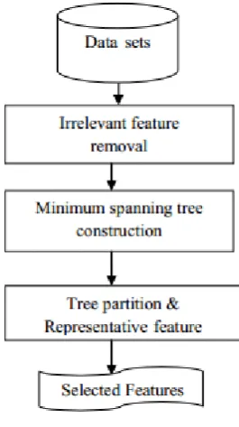
MST is a chart based model in creating the bunches from high computational multifaceted nature, it chooses or rejects the edges in MST. Traversing tree with their weight short of what or equivalent to the weight of each other crossing tree. Bunching by Minimal Spanning Tree can be view as a various levelled grouping calculation which track the divisive grouping methodology. Bunching calculation focused around least and greatest spreading over tree were by and large concentrated on to build MST of point set and erase clashing edges. Whose weights are expansively bigger than the standard weight of the nearby closeness edges in the tree? The objective to amplify the base buries group separation. MST based picture division is focused around select the edges from the diagram, where every pixel compare to a hub in the chart. Weights on every edge compute the disparity between pixels. The division calculation characterize the limitations between locales by looking at two amounts Intensity distinction over the limit and Intensity contrast between neighbouring pixels with all area[2]. This is valuable realizing that the force contrasts over the limit are paramount on the off chance that they are immense near to the fixation qualification inside the no less than one.

Figure 1: Least crossing tree

Above outline shows, unimportant gimmicks are expelled from given information sets, then develop the base traversing tree development and segment the tree to gather the delegate characteristics, from that agent characteristics we choose the pertinent peculiarities from MST.

3.3 Filter method

Channel technique - Filter techniques utilized as a substitute assess as an option of the mistake rate to get a gimmick subset. This measure is chosen to be quick to process. Basic methods in channel strategies are Mutual Information, association coefficient, and the entomb/intra class separation. Channels are normally less computationally thorough than wrappers, however channel delivers a list of capabilities which is doesn't tune to a definite sort of prescient model. Numerous channels manage the cost of a gimmick positioning instead of an unequivocal best peculiarity subset, and the cut-off point in the positioning is chosen through cross-approval [3] [4] [6].

3.4 Graph-theoretic clustering

Chart theoretic grouping are part vertices in a vast diagram into distinctive groups. Both coarse grouping and fine bunching are focused around this calculation called predominant set grouping. It delivers fine groups on inadequate high dimensional information space. This calculations that are held to execute well regarding the files clarify as in the past area are illustrated. The principal iteratively stress the intra-bunch over between group integration and the second is more than once refines a starting part focused around intra-bunch conductance. While together basically work by regional standards, we likewise propose an alternate, more worldwide strategy. In each of the three cases, the asymptotic most detrimental possibility running time of the calculations focused around specific parameters known as data. Be that as it may, see that for critical decisions of these parameters, the time intricacy of the novel calculation GM is better than for the other two calculations [8].

3.5 Feature selection

learning, detail and information mining groups. The principle target of gimmick choice is to pick a subset of data variables by disposing of peculiarities, which are superfluous or of no prescient data. Characteristic choice has demonstrated in both hypothesis and practice to be powerful in upgrading learning proficiency, expanding prescient exactness and lessening many-sided quality of scholarly comes about. Characteristic determination in regulated learning has a primary objective of discovering a gimmick subset that delivers higher arrangement exactness. As the dimensionality of an area stretches, the quantity of peculiarities N increments. Discovering an ideal peculiarity subset is recalcitrant and issues related gimmick determinations have been ended up being NP-hard. At this crossroads, it is crucial to portray customary peculiarity determination process, which comprises of four essential steps, to be specific, subset era, subset assessment, halting model, and approval.

Subset era is a pursuit prepare that creates hopeful gimmick subsets for assessment focused around a certain hunt methodology. Every applicant subset is assessed and contrasted and the past best one as indicated by a certain assessment [8] [9]. On the off chance that the new subset turns to be better, it replaces best one. This methodology is rehashed until a given halting condition is fulfilled. Positioning of peculiarities decides the criticalness of any individual peculiarity, ignoring their conceivable associations. Positioning systems are focused around detail, data hypothesis, or on a few capacities of classifier's yields.

Calculations for peculiarity determination fall into two general classes specifically wrappers that utilize the learning calculation itself to assess the value of peculiarities and channels that assess gimmicks as indicated by heuristics focused around general attributes of the information. A few legitimizations for the utilization of channels for subset determination have been examined and it has been accounted for that channels are nearly quicker than wrappers. Numerous understudy execution expectation models have been proposed and relative dissects of diverse classifier models utilizing Decision Tree, Bayesian Network, and other order calculations have likewise been examined .But, they uncover just classifier exactness without performing the peculiarity choice methodology [7].

3.6 Data source and prediction outcomes

Information SOURCE AND PREDICTION OUTCOMES School training in India is a two-level framework, the initial ten years covering general instruction emulated by two years of senior optional training. This two-year instruction, which is otherwise called Higher Secondary Education, is critical in light of the fact that it is an integral variable for picking craved subjects of study in higher training. Indeed, the higher auxiliary instruction goes about as an extension between school training and the higher learning specializations that are offered by schools and colleges. At this point, it is crucial to measure the scholastic execution of understudies, which is a testing undertaking because of the commitments of financial, mental and natural elements [4].

Estimation of scholastic execution is completed by utilizing the prescient models and it is to be noted that expectation demonstrating methodology are made out of a peculiarity extraction, which goes for safeguarding a large portion of the important gimmicks of understudy's qualities while avoiding any wellspring of unfriendly variability, and an order arrange that distinguishes the gimmick vector with proper class. Of course, the characterization operation focused around the

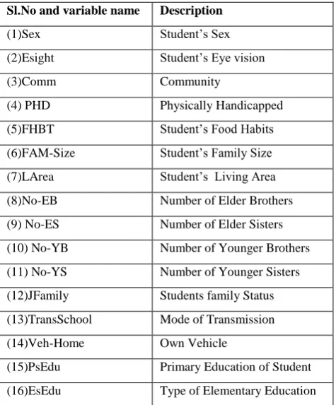
likelihood thickness capacity of the gimmick vector space is insufficient on account of unseemly decision of peculiarities [6], or in the vicinity of parameters, which don't give helpful data. In this manner, joining the arrangement process with gimmick choice strategy has turned into a need in the model development. The primary wellspring of information for this study is the reactions got from understudies through a poll with close-end questions. The reactions give demographic subtle elements, family points of interest, financial points of interest, past scholarly execution at optional level from distinctive schools and other ecological points of interest. A sum of 1969 higher auxiliary understudies from distinctive schools in diverse areas of the state Tamil Nadu, India, supplied the subtle elements. We recognize that the first peculiarity vector of understudy execution information comprised of 32 gimmicks that were prescient variables. Furthermore, there was a two-case class variable result (pass/ fall flat), which was considered as reaction variable. All these prescient and responsive variables indicated in Table 1 fit in with the sort of ostensible information[8] [9].

Table 1: Student Features subsets

Sl.No and variable name Description

(1)Sex Student’s Sex

(2)Esight Student’s Eye vision

(3)Comm Community

(4) PHD Physically Handicapped

(5)FHBT Student’s Food Habits

(6)FAM-Size Student’s Family Size

(7)LArea Student’s Living Area

(8)No-EB Number of Elder Brothers

(9) No-ES Number of Elder Sisters

(10) No-YB Number of Younger Brothers

(11) No-YS Number of Younger Sisters

(12)JFamily Students family Status

(13)TransSchool Mode of Transmission

(14)Veh-Home Own Vehicle

(15)PsEdu Primary Education of Student

(16)EsEdu Type of Elementary Education

Characteristic choice is typically done via looking the Space of quality subsets, assessing everyone. This is attained by joining trait subset evaluator with a pursuit strategy. In the present examination, an assessment of six channel characteristic subset routines with rank hunt or Greedy pursuit strategy was performed to discover the best capabilities [8].

1) Correlation-based Attribute assessment (CB),

2) Chi-Square Attribute assessment (CH),

3) Gain-Ratio Attribute assessment (GR),

4) Information-Gain Attribute assessment (IG),

5) Relief Attribute assessment (RF) and

These whole channel procedures said above could survey the significance of gimmicks [16] on the premise of the inborn properties of the information. Characteristic choice frequently builds classifier efficiency through the reduction of the span of the compelling peculiarities. Consequently, there is a need to confirm the pertinence of every last one of gimmicks in the peculiarity vector. In this association, we performed all the over six peculiarity choice systems focused around diverse measures to pick the best subsets for a given cardinality. We utilized hence the Naive Bayes arrangement Algorithm (calculation) [6][7], which is one of the most straightforward cases of probabilistic classifiers with precise conclusions as that of state-of-the art learning calculations for forecast model development, as a gauge classifier to choose the last best subset among the best subsets crosswise over diverse cardinalities. The measures like ROC Values and Macro-Average F1-Measure qualities are utilized within the present examination [5] [6].

4.

RESULTS AND DISCUSSION

The present examination concentrates on different peculiarity determination systems, which is a standout amongst the most essential and habitually utilized as a part of information pre-processing for information mining. The general techniques on Feature Selection as far as Filter strategy is taken after with the impact of peculiarity choice methods on a created database on higher auxiliary understudies. Viability of the calculations is displayed as far as diverse measures like ROC Values and Measure values. At first all gimmick choice strategies were connected on the first list of capabilities and the gimmicks were positioned as indicated by their benefits in rising request. Since no understanding was found among the gimmick positioning systems, we performed understudy execution assessment regarding ROC quality and F1-Measure values on numerous subsets of peculiarity vectors. Indeed, the assessment on the premise of ROC worth and F1-Measure was completed iteratively on the numerous subsets beginning from two with one as an augmentation from the positioning rundown [10] [9].

The Receiver Operating Characteristics (ROC) bend is a graphical representation of the exchange off between the false negative and false positive rates for each conceivable cut off. Identically, the ROC worth is the representation of the exchange offs in the middle of Sensitivity and Specificity. The assessment measures with varieties of ROC qualities and F1-Mesures are created from an Open Source Data Mining suite, WEKA that offers a thorough set of state-of-the-craftsmanship machine learning calculations and set of self-ruling gimmick determination and positioning strategies. The produced assessment measures are demonstrated in Fig. 1 for reference. While the X-axis represents the number of features,

Fig2: Measurement

The Y-axis represents the ROC value for each feature subset generated by six filter features. The maximum ROC value of all algorithms and the corresponding cardinalities from the Fig.1 are presented in Table 1. This is quite useful for fixing the optimal size of the feature subsets with the highest ROC values [4] [3].

Figure3: Feature Subset Comparison

The consequences of the similar investigation of four separate classifiers completed against gimmick subsets created by the five diverse peculiarity determination techniques are demonstrated in Fig. 3. Unmistakably all the four classifiers performed well for the peculiarity subset (IG-7) produced by data increase values. Additionally the classifiers Voted Perceptron, One R indicated high prescient exactness which is more than 89 percent. Specifically, the Voted Perceptron consistently gave the same level of prescient execution for all the peculiarity subsets. We see from the present investigation that, a wise blend of ROC qualities, F1-Measure, high Predictive Accuracy (PA) and low Root Mean Square Error (RMSE) for the IG strategy with main 7 peculiarities (i.e., IG-7), yields an ideal dimensionality of the list of capabilities[2] [1].

5.

CONCLUSION

In this paper, we did a similar investigation of six channel gimmick segment Algorithm (calculations) by which we could achieve the best technique and in addition ideal dimensionality of the peculiarity subset. Benchmarking of channel gimmick determination strategy was thusly completed by conveying distinctive classifier models. The aftereffects of the present study successfully upheld the well-known truth of expansion in the prescient exactness with the presence of least number of peculiarities. The normal results demonstrate a decrease in computational time and constructional cost in both preparing and grouping periods of the understudy execution model. In future to it can be applied to other classification forms along with the clusters.

6.

REFERENCES

[1] Johannes grabmeier andreas rudolph: Techniques of Cluster Algorithms in Data Mining May 23, 2001 Kluwer Academic Publishers. Manufactured in the Netherlands.

[3] YongSeog Kim, W. Nick Street, and Filippo Menczer: Feature Selection in Data Mining, University of Iowa, USA.

[4] M. Ramaswami and R. Bhaskaran: A Study on Feature Selection Techniques in Educational Data Mining journal of computing, volume 1, issue 1, december 2009, issn: 2151-9617.

[5] Tarek Amr: Survey on Feature Selection.

[6] Michael Abernethy: Data mining with WEKA, Part 2: Classification and clustering IBM.

[7] Marcos Evandro Cintra, Trevor P. Martin, Maria Carolina Monard, and Heloisa de Arruda Camargo:

Feature Subset Selection Using a Fuzzy Method 200 International Conference on Intelligent Human-Machine Systems and Cybernetics.

[8] Isabelle Guyon, Andre Elisseeff: An Introduction to Variable and Feature Selection, Journal of Machine Learning Research 3 (2003) 1157-1182.

[9] YongSeog Kim, W. Nick Street, and Filippo Menczer: Feature Selection in Data Mining,

University of Iowa, USA.

[10] Marie Gaudard: Interactive Data Mining and Design of Experiments: the JMP® Partition and Custom Design Platforms,March 2006 North Haven Group.