Two Dimensional Green's Function for a Half Space Geometry Due to Two Different Non-Integer Dimensional Spaces

(1)

Two Dimensional Green’s Function for a Half Space Geometry

due to Two Diﬀerent Non-Integer Dimensional Spaces

Muhammad A. Fiaz and Qaisar A. Naqvi*

Abstract—A two-dimensional Green’s function for a half space geometry, comprising planar interface only due to two different non-integer dimensional spaces, has been derived. Medium hosting the time harmonic electric line source and planar interface is homogeneous and isotropic. Radiated field is written in terms of unknown spectrum of plane waves. Unknown spectrum functions are determined using the related boundary conditions. It has been shown that although wavenumbers of two half spaces are same, due to difference of dimensions of the two half spaces, reflection and transmission occur. When dimensions of both half spaces are taken equal to two, derived expressions yield field radiated by a line source in an unbounded homogeneous medium with integer dimensional space.

1. INTRODUCTION

The concept and axiomatic basis for non-integer dimensional (NID) spaces was introduced by Strillinger [1]. However, recently derived solutions of the Helmholtz’s equation in NID spaces by Zubair et al. [2–7] have attracted the attention of researchers. Now concept of NID space is employed to study variety of problems related to electromagnetics. Reflection/transmission problems [8, 9], electrostatics, quasistatic and their application to plasmonic [10–12], Green’s function [13, 14], plasma [15], chiral metamaterial [16], scattering from buried cylinder [17], quantum-mechanics [18], Newtonian physics [19] and gravitational physics [20] in NID space were treated using these solutions. Continuous model for fractal medium, anisotropic fractal medium, flow of fractal fluids, vector calculus, fractal electrodynamics in NID spaces or using NID approach were studied by Tarasov [21–27]. According to Tarasov [28], non-integer dimensional space allows to describe fractal media in the frame work of continuum model. Here, expressions for Green’s function reported in [29] are derived for NID interface.

In all previous discussions available in published literature, NID-space geometries with interface were considered, but the interface, in each case, is due to two different mediums. In addition, one or both sides of the interface were NID. In present discussion, it has been assumed that the cause of interface is only the difference of values of dimension of the NID spaces whereas wavenumber of the two half spaces is same. The purpose of current discussion is to derive a two-dimensional Green’s function for half space, occurring due to difference in values of the dimension of two NID spaces when mediums of the two half spaces have same wavenumber. The derived Green’s functions may be used in the study of buried object detection. Theoretical formulation of the problem is given in Section 2 while numerical results are reported in Section 3.

2. FORMULATION

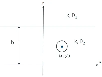
Consider an NID half-space geometry with planar interface located at y = b as shown in Figure 1. Both half spaces of the geometry are ﬁlled with the medium having same wavenumber but diﬀerent

Received 10 January 2018, Accepted 18 March 2018, Scheduled 27 March 2018

* Corresponding author: Qaisar Abbas Naqvi ([email protected]).

(2)

Figure 1. Geometry of the problem. A fractal-fractal interface is considered.

dimensions. Wavenumber of the medium is k=ω√μ. That is, medium is homogeneous, lossless and isotropic. Region y > bis termed upper half-space, and region y < b is called lower half-space. Both half spaces are taken as non-integer dimension along y-direction of the Cartesian coordinate system. Non-integer dimensions of upper half-space and lower half-space are denoted asD1 andD2, respectively.

A line source carrying time harmonic electric current is located at (x, y) in lower NID half space. The geometry is divided into three regions. Upper half-space is called region I, y < y < b termed region II, and y < y termed region III. In three regions of the geometry, unknown ﬁelds radiated by the line source may be written in terms of the spectrum of uniform plane waves.

Electric ﬁeld in terms of spectrum of plane waves for each region may be written as [14, 17]

E1z(x, y;x, y) =

_∞

−∞A(kx) exp(ikxx)(kyy)

n1_H(1)

n1 (kyy)dkx, y > b (1)

E2z(x, y;x, y) =

_∞

−∞B(kx) exp(ikxx)(kyy)

n2_H(1)

n2(kyy)dkx

+

_∞

−∞C(kx) exp(ikxx)(kyy)

n2_H(2)

n2 (kyy)dkx, y < y < b (2)

E3z(x, y;x, y) =

_∞

−∞D(kx) exp(ikxx)(kyy)

n2_H(2)

n2(kyy)dkx, y < y (3)

where A(·), B(·), C(·) and D(·) are unknown spectrum functions to be determined. y-component of the wave vector is ky = k2−k2x. Hn(1)1 (·) is the Hankel function of ﬁrst kind and non-integer order.

Hn(2)2 (·) is the Hankel function of second kind and non-integer order. Non-integer order of the Hankel

function isni = 3−₂Di,i= 1,2 with 1< Di≤2.

Corresponding magnetic field may be obtained using the Ampere’s Maxwell curl postulate. In order to apply the boundary conditions, tangential component of the magnetic field is also required. It is obvious from the geometry that x-component of the magnetic field is tangential to the interface. Component of magnetic field tangential to the interface is given below

H1x(x, y;x, y) = − i

ωμ ∂Ez

∂y −

i ωμ

1 2

D1−2

y Ez

= − i ωμ

_∞

−∞kyA(kx) exp(ikxx)(kyy)

n1_H(1)

n1h(kyy)dkx (4)

H2x(x, y;x, y) = − i

ωμ

_∞

−∞kyB(kx) exp(ikxx)(kyy)

n2_H(1)

n2h(kyy)dkx

+ i ωμ

_∞

−∞kyC(kx) exp(ikxx)(kyy)

n2_H(2)

(3)

H3x(x, y;x, y) = i

ωμ

_∞

−∞kyD(kx) exp(ikxx)(kyy)

n2_H(2)

n2h(kyy)dkx (6)

where

H_n(1)₁_h(kyy) = H_n(1)₁₋1(kyy)−

1 2

D1−1

kyy H

(1)

n1 (kyy)

H_n(1)₂_h(kyy) = Hn(1)2−1(kyy) +

1 2

D2−1

kyy H

(1)

n2 (kyy)

H_n(2)₂_h(kyy) = Hn(2)2−1(kyy) +

1 2

D2−1

kyy H

(2)

n2 (kyy)

There are two interfaces in the geometry located at y = b and y = y. Boundary conditions at interfacey =bare

E1z(x, b;x, y) = E2z(x, b;x, y) (7)

∂E1z(x, y;x, y)

∂y −

1 2

D1−2

y E1z

y=b

= ∂E2z(x, y;x

_{, y}₎

∂y −

1 2

D2−2

y E2z

y=b

(8)

At interface y=y where line source is located, ﬁelds must satisfy following conditions

E2z(x, b;x, y) =E3z(x, b;x, y) (9)

∂E1z(x, y;x, y)

∂y

y=y

− ∂E2z(x, y;x, y)

∂y

y=y

=iωμI0δ(x−x) (10)

Using above boundary conditions, unknown spectrum functions can be determined. Unknown spectrum functionsA(·),B(·),C(·) andD(·) are given below

A(kx) = iωμI0 2π

exp(−ikxx) ky(kyy)n2

Hn(2)2 (kyy)

Hn(1)2 (kyy)H

(2)

n2h(kyy)−H

(2)

n2 (kyy)H

(1)

n2h(kyy)

×(kyb)n2

(kyb)n1

Hn(2)2(kyb)H

(1)

n2h(kyb)−H

(1)

n2(kyb)H

(2)

n2h(kyb)

−Hn(1)1(kyb)H

(2)

n2h(kyb) +H

(2)

n2 (kyb)H

(1)

n1h(kyb)

B(kx) = iωμI₂_π 0exp(−ikxx

₎

ky(kyy)n2

Hn(2)2 (kyy)

Hn(1)2 (kyy)H

(2)

n2h(kyy)−H

(2)

n2 (kyy)H

(1)

n2h(kyy)

C(kx) = iωμI₂ 0 π

Hn(2)2 (kyy)

Hn(1)2 (kyy)H

(2)

n2h(kyy)−H

(2)

n2 (kyy)H

(1)

n2h(kyy)

× H (1)

n1(kyb)H

(1)

n2h(kyb)−H

(1)

n2(kyb)H

(1)

n1h(kyb)

−Hn(1)1(kyb)H

(2)

n2h(kyb) +H

(2)

n2 (kyb)H

(1)

n1h(kyb)

D(kx) = iωμI₂_π 0exp(−ikxx

₎

ky(kyy)n2

Hn(1)2 (kyy)

Hn(1)2 (kyy)H

(2)

n2h(kyy)−H

(2)

n2 (kyy)H

(1)

n2h(kyy)

+C(kx)

In the next section, spectrum functions have been derived from the above results when both half spaces are of integer dimension. Then special cases of the above geometry have been derived by assuming that one of the two half spaces is of non-integer dimension.

2.1. Special Cases

(4)

n1h =n2h =−1₂. The resulting expressions for unknown coeﬃcients are [See Appendix of 17]

A(kx) = −iωμI0 4π

π 2

exp(−ikxx−ikyy) ky

B(kx) = −iωμI₄_π 0

π 2

C(kx) = 0

D(kx) = −iωμI0 4π

π 2

exp(−ikxx+ikyy) ky

These are well known results for a line source located in unbounded integer dimensional space having wavenumberk. Now consider the two interesting cases, in each case only one half space is of non-integer dimension.

2.1.1. Case 1: Upper Half-Space is NID

In this case the upper half-space is NID whereas the lower half-space is of integer dimension. Therefore D2= 2, n2= 1₂ and n2h=−1₂. The resulting expressions for unknown coeﬃcients become

A(kx) = −iωμI0 2π

exp(−ikxx−ikyy) (kyb)n1

exp(ikyb)

−ikyHn(1)1 (kyb) +kyH

(1)

n1h(kyb)

B(kx) = −iωμI₄ 0 π

π 2

C(kx) = iωμI₄_π0

π 2

Hn(1)1(kyb) +iH

(1)

n1h(kyb) Hn(1)1(kyb)−iH

(1)

n1h(kyb)

exp(2ikyb)

D(kx) = −iωμI0 4π

π 2

exp(−ikxx+ikyy)

ky +C(kx)

2.1.2. Case 2: Lower Half-space is NID

In this case the lower half-space is of non-integer dimension whereas the upper half-space is of integer dimension. Therefore,D1= 2, n1 = 1₂ and n1h =−1₂ are taken. The resulting expressions for unknown

coeﬃcients become

A(kx) = −ωμI₂_π0

π 2

exp(−ikxx−ikyb) ky(kyy)n2 ×

Hn(2)2 (kyy)

Hn(1)2 (kyy)H

(2)

n2h(kyy)−H

(2)

n2(kyy)H

(1)

n2h(kyy)

×(kyb)n2H

(2)

n2(kyb)H

(1)

n2h(kyb)−H

(1)

n2(kyb)H

(2)

n2h(kyb)

−Hn(2)2h(kyb) +iH

(2)

n2(kyb)

B(kx) = iωμI0 2π

Hn(2)2(kyy)

Hn(1)2(kyy)H

(2)

n2h(kyy)−H

(2)

n2 (kyy)H

(1)

n2h(kyy)

C(kx) = iωμI₂_π0exp(−ikxx

₎

ky(kyy)n2

Hn(2)2(kyy)

Hn(1)2(kyy)H

(2)

n2h(kyy)−H

(2)

n2 (kyy)H

(1)

n2h(kyy)

× H (1)

n2h(kyb)−iH

(1)

n2(kyb)

−Hn(2)2h(kyb) +iH

(2)

n2 (kyb)

D(kx) = iωμI0 2π

−Hn(1)2(kyy)

Hn(1)2(kyy)H

(2)

n2h(kyy)−H

(2)

n2 (kyy)H

(1)

n2h(kyy)

(5)

2.2. Asymptotic Analysis

In this section, far-zone ﬁeld expression is derived taking large value of the observation distance. Field expression for region I taking only lower half-space as NID is given below

E1z = iωμI0

4π

_∞

−∞

exp(−ikxx−ikyb) ky(kyy)n2 ×

Hn(2)2(kyy)

Hn(1)2(kyy)H

(2)

n2h(kyy)−H

(2)

n2(kyy)H

(1)

n2h(kyy)

×(kyb)n2H

(2)

n2(kyb)H

(1)

n2h(kyb)−H

(1)

n2(kyb)H

(2)

n2h(kyb)

−Hn(2)2h(kyb) +iH

(2)

n2 (kyb)

exp{ikxx+ikyy}dkx (11)

Setting

x = ρcosφ, y=ρsinφ kx = kcosθ, ky =ksinθ

x = ρcosφ, y=ρsinφ

Stationary point is located at θ=φ. Applying the method of stationary phase [30] by taking kρ→ ∞ yields

E1z(ρ, φ;ρ, φ) ∼ iωμI0

2√2π

exp(ikρ−iπ/4)

√

kρ

exp(−ikρcosφcosφ−ikbsinφ) (kρsinφsinφ)n2

× H

(2)

n2(kρsinφsinφ)

Hn(1)2 (kρsinφsinφ)H

(2)

n2h(kρsinφsinφ)−H

(2)

n2 (kρsinφsinφ)H

(1)

n2h(kρsinφsinφ)

×(kbsinφ)n2H

(2)

n2(kbsinφ)H

(1)

n2h(kbsinφ)−H

(1)

n2(kbsinφ)H

(2)

n2h(kbsinφ)

−Hn(2)2h(kbsinφ) +iH

(2)

n2 (kbsinφ)

(12)

Field expression for region below the line source, taking only upper half-space as NID, is given below

E3z = iωμI0

4π

_∞

−∞

1 ky exp

ikx(x−x)−iky(y+y)

+H

(1)

n1 (kyb) +iH (1)

n1h(kyb)

H_n(1)1 (kyb)−iH (1)

n1h(kyb)

1

ky exp (i2kyb) exp

ikx(x−x)−iky(y−y) dkx (13)

Stationary point is located at θ = −φ. Applying the method of stationary phase [30] by taking kρ→ ∞ yields

E3z(ρ, φ;ρ, φ) ∼ iωμI0

2√2π

exp(ikρ−iπ/4)

√

kρ

exp−ikρcos(φ−φ)

+H

(1)

n1(−kbsinφ)+iH (1)

n1h(−kbsinφ)

H_n(1)1(−kbsinφ)−iH (1)

n1h(−kbsinφ)

exp(−i2kbsinφ) exp−ikρcos(φ+φ) (14)

whereπ < φ <2π.

3. NUMERICAL RESULTS

To validate the expression, it can be assumed thatD1=D2. The expressions are reduced to well-known

case of a line source radiating in a dielectric medium as discussed in Section 2.2. Asymptotic solution of the problem has been given in Equation (12) while lower half space is considered NID. Figure 2 shows the radiation pattern for different values of D2. It can be observed that NID has significant effect on

pattern even if dielectric properties of the two fractals are same. As D2 → 2, the pattern shows little

(6)

value ofbincreases, i.e., the separation between interface and the source increases which results in small reﬂection by interface, and the radiation in region I increases. It has been checked that radiation does not increase beyond limits and must satisfy radiation condition. Moreover, it is a complex function of b and D2 described by Equation (12). To further analyze, the radiation pattern as a function of b

for diﬀerent values of D2 is shown in Figure 4. It decreases as D2 increases and becomes constant for

0 20 40 60 80 100 120 140 160 180

φ

2.2

2

1.8

1.6

1.4

1.2

1

0.8

|

E

|

1

z

D = 1.4

D = 1.6

D = 1.8

2 2 2

Figure 2. Radiation pattern in region I for diﬀerent values of D1 whereb= 0.4.

0 20 40 60 80 100 120 140 160 180

φ

2.2

2

1.8

1.6

1.4

|

E

|

1

z

b = 0.4

b = 0.6

b = 0.8 2.4

2.6 2.8 3

Figure 3. Radiation pattern in region I for diﬀerent values ofb, whereD2 = 1.4.

0 1 2 3 4

5

4.5

5

3.5

3

2.5

2

1.5

|

E

|

1

z

D = 1.1

D = 1.4

D = 1.7

2 2 2

D 2= 2

b 1

0.5

Figure 4. Radiation pattern in region I as a function of bfor diﬀerent values of D2.

180 200 220 240 260 280 300 320 340 360

φ

1.75

1.7

1.65

1.6

1.55

1.5

1.45

1.4

|

E

|

3

z D = 1.4

D = 1.6 D = 1.8

1 1 1

1.35

Figure 5. Radiation pattern in region III for diﬀerent values ofD1 whereb= 0.4.

180 200 220 240 260 280 300 320 340 360

φ

1.75

1.7

1.65

1.6

1.55

1.5

1.45

1.4

|

E

|

3

z

1.35

b = 0.4

b = 0.6

b = 0.8

(7)

integer dimensionsD2 = 2. For all the simulation, it is assumed that ρ = 0.2,φ = 30◦, and r= 4.

Asymptotic solution of the problem can also be obtained by taking the upper half space as NID. It has been given in Equation (14). Figure 5 shows the radiation pattern for diﬀerent values of D1.

Again for D1 →2, the pattern shows very small variations for all the angles, and it approaches that of

line source radiating in a dielectric medium for D1 = 2. Radiation pattern for diﬀerent values of b is

shown in Figure 6. It can be observed that the location of interface has some role to play in the case of fractals.

4. CONCLUSION

Half space geometry resulting from two different NID-spaces is studied when it is excited by a current carrying line source. Reflected and transmitted fields due to NID-interface are determined using the boundary conditions on fields. Well-known results, line source in an unbounded integer dimensional space, are reproduced as a special case. Although wavenumbers of the two half spaces are the same, difference of dimensions of the two half spaces yields reflection of the radiated field from the interface.

REFERENCES

1. Stillinger, F. H., “Axiomatic basis for spaces with non-integer dimensions,”Journal of Mathematical Physics, Vol. 18, 1224–1234, 1977.

2. Zubair, M., M. J. Mughal, and Q. A. Naqvi,Fractional Fields and Waves in Fractional Dimensional Space, Springer-Verlag, New York (NY), 2012.

3. Zubair, M., M. J. Mughal, and Q. A. Naqvi, “The wave equation and general plane wave solution in fractional space,” Progress In Electromagnetics Research Letters, Vol. 19, 137–146, 2010. 4. Zubair, M., M. J. Mughal, and Q. A. Naqvi, “An exact solution of cylindrical wave equation

for electromagnetic ﬁeld in fractional dimensional space,” Progress In Electromagnetics Research, Vol. 114, 443–455, 2011.

5. Zubair, M., M. J. Mughal, and Q. A. Naqvi, “An exact solution of spherical wave in D-dimensional fractional space,”Journal of Electromagnetic Waves and Applications, Vol. 25, No. 10, 1481–1491, 2011.

6. Zubair, M., M. J. Mughal, and Q. A. Naqvi, “On electromagnetic wave propagation in fractional space,”Nonlinear Analysis: Real World Applications, Vol. 12, 2844–2850, 2011.

7. Zubair, M., M. J. Mughal, Q. A. Naqvi, and A. A. Rizvi, “Diﬀerential electromagnetic equations in fractional space,” Progress In Electromagnetics Research, Vol. 114, 255–269, 2011.

8. Asad, H., M. Zubair, and M. J. Mughal, “Reﬂection and transmission at dielectric-fractal interface,” Progress In Electromagnetics Research, Vol. 125, 543–558, 2012.

9. Attiya, A. M., “Reﬂection and transmission of electromagnetic wave due to a quasi-fractional-space slab,”Progress In Electromagnetics Research Letters, Vol. 24, 119–128, 2011.

10. Baleanua, D., A. K. Golmankhaneh, and A. K. Golmankhaneh, “On electromagnetic ﬁeld in fractional space,” Nonlinear Analysis: Real World Applications, Vol. 11, 288–292, 2010.

11. Naqvi, Q. A. and M. Zubair, “On cylindrical model of electrostatic potential in fractional dimensional space,” Optik-International Journal for Light and Electron Optics, Vol. 127, 3243– 3247, 2016.

12. Noor, A., A. A. Syed, and Q. A. Naqvi, “Quasi-static analysis of scattering from a layered plasmonic sphere in fractional space,” Journal of Electromagnetic Waves and Applications, Vol. 29, No. 8, 1047–1059, 2015.

13. Asad, H., M. J. Mughal, M. Zubair, and Q. A. Naqvi, “Electromagnetic Green’s function for fractional space,” Journal of Electromagnetic Waves and Applications, Vol. 26, Nos. 14–15, 1903– 1910, 2012.

(8)

15. Zubair, M. and L. K. Ang, “Fractional-dimensional Child-Langmuir law for a rough cathode,” Physics of Plasmas (1994-present), Vol. 23, 072118, 2016.

16. Hameed, A., M. Omar, A. A. Syed, and Q. A. Naqvi, “Power tunneling and rejection from fractal chiral-chiral interface,”Journal of Electromagnetic Waves and Applications, Vol. 28, No. 14, 1766– 1776, 2014.

17. Abbas, M., A. A. Rizvi, A. Fiaz, and Q. A. Naqvi, “Scattering of electromagnetic plane wave from a low contrast circular cylinder buried in non-integer dimensional half space,” Journal of Electromagnetic Waves and Applications, Vol. 31, No. 3, 263–283, 2017.

18. Sandev, T., I. Petreska, and E. K. Lenzi, “Harmonic and anharmonic quantum-mechanical oscillators in non-integer dimensions,”Phys. Lett. A, Vol. 378, 109–116, 2014.

19. Palmer, C. and P. N. Stavrinou, “Equations of motion in a non-integer-dimensional space,”Journal of Physics A: Mathematical and General, Vol. 37, 2004.

20. Muslih, S., D. Baleanu, and E. Rabei, “Gravitational potential in fractional space,”Open Physics, Vol. 5, 285–292, 2007.

21. Tarasov, V. E., “Continuous medium model for fractal media,” Phys. Lett. A, Vol. 336, 167–174, 2005.

22. Tarasov, V. E., “Anisotropic fractal media by vector calculus in non-integer dimensional space,” Journal of Mathematical Physics, Vol. 55, 083510, 2014.

23. Tarasov, V. E., “Elasticity of fractal materials using the continuum model with non-integer dimensional space,”Comptes Rendus Mecanique, Vol. 343, 57–73, 2015.

24. Tarasov, V. E., “Flow of fractal ﬂuid in pipes: Non-integer dimensional space approach,” Chaos, Solitons and Fractals, Vol. 67, 26–37, 2014.

25. Tarasov, V. E., “Vector calculus in non-integer dimensional space and its applications to fractal media,” Communications in Nonlinear Science and Numerical Simulation, Vol. 20, 360–374, 2015. 26. Tarasov, V. E., “Electromagnetic waves in non-integer dimensional spaces and fractals,” Chaos,

Solitons and Fractals, Vol. 81, 38–42, 2015.

27. Tarasov, V. E., “Fractal electrodynamics via non-integer dimensional space approach,”Phys. Lett. A, Vol. 379, 2055–2061, 2015.

28. Tarasov, V. E., “Acoustic waves in fractal media: Non-integer dimensional spaces approach,”Wave Motion, Vol. 63, 18–22, 2016.

29. Naqvi, Q. A. and A. A. Rizvi, “Scattering from a cylindrical object buried in a geometry with parallel interfaces,” Progress In Electromagnetics Research, Vol. 27, 19–35, 2000.