PERFORMANCE ANALYSIS OF QPSK MODULATION
SCHEMES USING GRAY & NAIVE CODING WITH
RAYLEIGH FADING CHANNEL
1Biswajit Basak, 2Mousumi De
1
Assistant Professor
,
Dept o f ECE, Hooghly Engg. &Technology College, Hooghly, (India)
2M.Tech student, Microwave & Communication Engg., MCKV Institute of Engineering, Howrah, (India)
ABSTRACT
Orthogonal Frequency Division Multiplexing (OFDM) using Quadrature Amplitude system keying is a very common
approach in multi carrier communication. In this paper, we have shown a comparative analysis between the GRAY
and NAÏVE QPSK scheme with OFDM in both AWGN and Rayleigh fading channel. We have chosen the parameters
BER vs SNR for Gray and naïve and Rayleigh for the performance analysis as these two are the most important
parameter for any wireless communications.
Keywords: OFDM, GRAY, NAÏVE, QPSK, AWGN, BER, SNR
I.INTRODUCTION
OFDM has its major benefits of higher data rates and better performance. High data rates are achieved by the use of multiple carriers and performance improvement is caused by the use of guard interval thus mitigating ISI. In many wideband cellular systems, the channel experiences frequency selective fading In this paper we present the BER analysis of QPSK-OFDM systems over Rayleigh fading channel. Our Technical contributions are summarized below .We express the average SNR in terms Vs BER with gray and naïve code and Rayleigh fading channel.
1.1 QPSK
In QPSK, the data bits to be modulated are grouped into symbols, each containing two bits, and each symbol can take on one of four possible values: 00, 01, 10, or 11. During each symbol interval, the modulator shifts the carrier to one of four possible phases corresponding to the four possible values of the input symbol. In the ideal case, the phases are each 90 degrees apart, and these phases are usually selected such that the signal constellation. This structure uses the trigonometric identity
θ=tan−1(Q/I) (3)
If the output of this modulator is to be represented in complex-envelope form referenced to the carrier frequency, the modulated signal is given simply as
̃ x(t)=I(t)+jQ(t) (4) Simulation of this idealized signal requires only a trivial model of the modulator. The complex signal
̃x(t)is formed by simply using the in phase baseband signal I(t) as the real part and the quadrature baseband signal Q(t) as the imaginary part.
1.2 GRAY CODE
The reflected binary code, also known as Gray code after Frank Gray, is a binary numeral system where two successive values differ in only one bit. The reflected binary code was originally designed to prevent spurious output from electromechanical switches. Today, Gray codes are widely used to facilitate error correction in digital communications such as digital terrestrial television and some cable TV systems.
An n-bit Gray code, also called there reflected binary code, is an ordering of the 2n strings of length n over{0,1}such that every pair of successive strings differ in exactly one position.
Instead of the usual binary representation, we see that incrementing a number by one involves flipping only one bit. In the usual binary representation, incrementing by 1 could lead to a sequence of bits that are carried over, which may change several consecutive bits at once.
1.3 NAIVE CODE
This section formally states the assumptions and notations and recalls the naive Bayes and selective naive Bayes approaches.
Assumptions and Notation:
Let X = (X1;X2; : : :XK) be the vector of the K explanatory variables and Y the class variable. Let λ1; λ2; : : : λJbe the
J class labels of Y.
Let N be the number of instances and D = {D1;D2;……;DN} the labeled database containing the
instances Dn = (x(n); y(n)).Let M = {Mm}be the set of all the potential selective naive Bayes models. Each model Mm
is described by K parameter values amk, where amkis 1 if variable k is selected in model Mm and 0 otherwise. Let us denote by P(λj) the prior probabilities P(Y = λj) of the class values, and by P(Xk׀λj)
the conditional probability distributions P(Xk׀Y = lj) of the explanatory variables given the class values. We assume that the prior probabilities P(λj) and the conditional probability distributions
P(Xk׀λj) are known, once the preprocessing is performed.
In the experimental section, the P(λj) are estimated by counting and the P(Xk׀λj) are computed using the contingency
tables, resulting from the preprocessing of the explanatory variables. The conditional probabilities are estimated using a m-estimate (support +mp)=(coverage+m) with m = J=N and
1.3.1 Naive Bayes Classifier
The naive Bayes classifier assigns to each instance the class value having the highest conditional probability
P(jjX) =P(j)P(Xjj) /P(X) (5)
Using the assumption that the explanatory variables are independent conditionally to the class variable, we get
P(jjX) =P(j)Kk=1 P(Xkjj)/P(X) (6)
In classification problems, Equation (6) is sufficient to predict the most probable class given the input data, since
P(X) is constant. In problems where a prediction score is needed, the class conditional probability can be estimated using
P(jjX) = P(j)Kk =1 P(Xkjj)/Ji=1 P(i)Kk=1 P(Xkji) (7)
The naive Bayes classifier is poor at predicting the true class conditional probabilities, since the independence assumption is usually violated in real data applications. However, Hand and Yu (2001) show that the prediction score given by Equation (7) often provides an effective ranking of the instances for each class value.
II.ANALOGY BETWEEN SPECTRAL BROADENING IN FADING AND SPECTRAL
BROADENING IN KEYING A DIGITAL SIGNAL
Let us discuss the reason why a signal experiences spectral broadening as it propagates from, or is received by, a moving platform, and why this spectral broadening (also called the fading rate of the channel) is a function of the speed of motion. An analogy can be used to explain this phenomenon. Figure 3 shows the keying of a digital signal (such as amplitude shift keying or frequency shift keying), where a single tone cos2Πfct defined for – ∞ < t < ∞ is
Figure1: Analogy between spectral broadening in fading and spectral broadening in keying a
digital signal
III.FLOWCHART
It is clear that the amplitude has a Rayleigh distribution and that the phase has a uniform distribution when we observe the received signal at the arrival time. It is also clear that there are fixed ratios of the average electric powers of the direct and delayed waves.
For delayed wave #j
Shift of input data by delayed time
Fade for the shifted signal by sub function
j =the number of
delayed wave Start j= 0
That is to say, we have only to give the relative signal level and relative delay time of delayed waves in comparison with the direct wave, when this multipath propagation environment is simulated
IV.SIMULATION RESULTS AND DISCURSSION
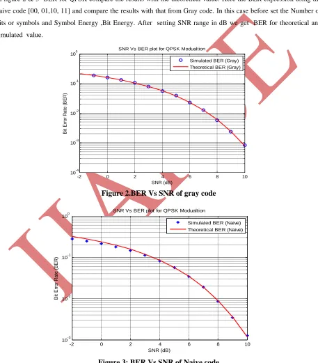
In figure 2 & 3 BER for QPSK compare the results with the theoretical value. Here the BER expression using the naive code [00, 01,10, 11] and compare the results with that from Gray code. In this case before set the Number of bits or symbols and Symbol Energy ,Bit Energy. After setting SNR range in dB we get BER for theoretical and simulated value.
Figure 2.BER Vs SNR of gray code
Figure 3: BER Vs SNR of Naive code
-2 0 2 4 6 8 10
10-4 10-3 10-2 10-1 100 SNR (dB) B it E rr o r R a te ( B E R )
SNR Vs BER plot for QPSK Modualtion
Simulated BER (Gray) Theoretical BER (Gray)
-2 0 2 4 6 8 10
10-3 10-2 10-1 100 SNR (dB) B it E rr o r R a te ( B E R )
SNR Vs BER plot for QPSK Modualtion
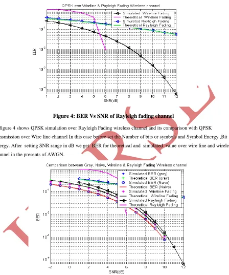
Figure 4: BER Vs SNR of Rayleigh fading channel
In figure 4 shows QPSK simulation over Rayleigh Fading wireless channel and its comparison with QPSK transmission over Wire line channel In this case before set the Number of bits or symbols and Symbol Energy ,Bit Energy. After setting SNR range in dB we get BER for theoretical and simulated value over wire line and wireless channel in the presents of AWGN.
Figure 5:BER Vs SNR in GRAY, NAÏVE, Wireline & Rayleigh Fading Channel
In figure 5 shows GRAY NAÏVE AND QPSK simulation and Rayleigh Fading wireless channel
V.CONCLUSION
From the simulation results the clear comparison between GRAY NAÏVE and RAYLEIGH FADING CHANNEL is shown and also the BER Vs SNR also is shown here in figure 5.Here the different theoretical BER and SNR and also simulated BER ,SNR compared as the given same no of bit, bit energy, symbol energy and also same the SNR range in db.
REFERENCES
[1] Jun Lu, Thiang Tjhung,Fumiyuki Adachi and Cheng Li Huang, “BER performance of OFDM-MDPSK system in Frequency -Selective Rician Fading with Diversity
[2] T.Wang, J. G. Proakis, E. Masry, and J. R. Zeidler, “Performance degradation of OFDM systems due to Doppler spreading,” IEEE Trans. Wireless Commun., vol. 5, no. 6, pp. 1422–1432, Jun. 2006.
[3] F. Gray. Pulse code communication, March 17, 1953 (filed Nov. 1947). U.S. Patent 2,632,058
[4] Jian Li, Xian-Da Zhang, Qiubin Gao,Yajuan Luo, Daqing Gu, “ Exact BEP Analysis for Coherent M-ary PAM and QAM over AWGN and Rayleigh Fading Channels,” Vehicular Technology Conference,2008.VTC Spring 2008,IEEE,Digital Object Identifier 10.1109/VETECS.2008.93, 14 May 2008 pp: 390 - 394
[5] David Tse, Pramod Viswanath, “Fundamentals of Wireless Communication” ch 2.4.2, Cambridge university press, 1st ed., pp- 34-37,2005.
[6] John R. Barry, Edward A. Lee, David G. Messerschmitt “Digital Communication, ”Kluwer academic publishers , 3rd ed. ch-5,pp- 164-184,2003.
[7]Guyon, A.R. Saffari, G. Dror, and J.M. Bumann. Performance prediction challenge. In International Joint Conference on Neural Networks, pages 2958–2965, 2006c.
[8]D.J. Hand and K. Yu. Idiot bayes ? not so stupid after all? International Statistical Review, 69(3): 385–399, 2001. [9]J.A. Hoeting, D. Madigan, A.E. Raftery, and C.T. Volinsky. Bayesian model averaging: A tutorial.
Statistical Science, 14(4):382–417, 1999. .
Biswajit Basak received the M.E. degree in CSE from WBUT in 2007. He worked as Asst. Professor in Hooghly Engineering & Technology College, Hooghly,W.B, India.His research interest include VLSI Design, Wireless Communication.He has published quite a few Research papers in International conferences. For further correspondence his e-mail is
Mousumi De received the B.E. degree in AEIE from the Burdwan University of