An Information Gain-Driven Feature Study for
Aspect-Based Sentiment Analysis
Kim Schouten, Flavius Frasincar, and Rommert Dekker Erasmus University Rotterdam
Burgemeester Oudlaan 50, 3062 PA Rotterdam, the Netherlands
{schouten, frasincar, rdekker}@ese.eur.nl
Abstract. Nowadays, opinions are a ubiquitous part of the Web and sharing experiences has never been more popular. Information regarding consumer opinions is valuable for consumers and producers alike, aiding in their respective decision processes. Due to the size and heterogeneity of this type of information, computer algorithms are employed to gain the required insight. Current research, however, tends to forgo a rigorous analysis of the used features, only going so far as to analyze complete feature sets. In this paper we analyze which features are good predictors for aspect-level sentiment using Information Gain and why this is the case. We also present an extensive set of features and show that it is possible to use only a small fraction of the features at just a minor cost to accuracy.
Keywords: Sentiment Analysis, Aspect-Level Sentiment Analysis, Data Mining, Feature Analysis, Feature Selection, Information Gain
1
Introduction
Nowadays, opinions are a ubiquitous part of the Web and sharing experiences has never been more popular [4]. Information regarding consumer opinions is valuable for consumers and producers alike, aiding in their respective decision processes. Due to the size and heterogeneity of this type of information, com-puter algorithms are employed to gain insight into the sentiment expressed by consumers and on what particular aspects that sentiment is expressed, and re-search into this type of algorithms has enjoyed increasingly high popularity over the last decade [8].
Research has led to a number of different approaches to aspect-level senti-ment analysis [13], that can be divided into three categories. The first group consists of methods that predominantly use a sentiment dictionary (e.g., [6]). Sentiment values are then assigned to certain words or phrases that appear in the dictionary and using a few simple rules (e.g., for negation and aggregation), the sentiment values are combined into one score for each aspect. The second type is categorized by the use of supervised machine learning methods (e.g., [3]). Using a significant amount of annotated data, where the sentiment is given for
each aspect, a classifier can be trained that can predict the sentiment value for yet unseen aspects. Last, some methods based on unsupervised machine learn-ing are also available, but these usually combine aspect detection and sentiment classification into one algorithm (e.g., [14]).
Supervised learning has the advantage of high performance, and given the fact that sentiment is usually annotated as a few distinct classes (i.e., positive, neutral, and negative), traditional statistical classifiers work remarkably well. Unfortunately, most of these methods are somewhat of a black box: once provided with enough input, the method will do its task and will classify aspect sentiment with relatively good accuracy. However, the inner workings are often unknown, and because of that, it is also not known how the various input features relate to the task. Since most classifiers can deal with large dimensionality on the input, one tends to just give all possible features and let the classifier decide which ones to use. While this is perfectly fine when aiming for performance, it does not give much insight into which particular features are good predictors for aspect sentiment. Knowing which features are relevant is important for achieving insight into the performed task, but it also allows to speed up the training process by only employing the relevant features with possibly only a minor decrease in performance.
This focus on performance instead of explanation is most typically found in benchmark venues, such as the Semantic Evaluation workshops [12]. Here, participants get annotated training data and are asked to let their algorithm provide the annotations for a non-annotated data set. The provided annotations are then centrally evaluated and a ranking is given, showing how each of the participating systems fared against each other. Scientifically speaking, this has the big benefit of comparability, since all of the participants use the same data and evaluation is done centrally, as well as reproducibility, since the papers published in the workshop proceedings tend to focus on how the system was built. The one thing missing, however, is an explanation of why certain features or algorithms perform so great or that bad, since there usually is not enough space in the allowed system descriptions to include this.
Hence, this paper aims to provide insight into which features are useful, using a feature selection method based on Information Gain [11], which is one of the most popular feature filtering approaches. Compared to wrapper approaches, such as Forward Feature Selection, it does not depend on the used classification algorithm. Using Information Gain, we can compute a score for each individual feature that represents how well that feature divides the aspects between the various sentiment classes. Thus, we can move beyond the shallow analysis done per feature set, and provide deeper insight, on the individual feature level.
The remainder of this paper is organized as follows. First, the problem of aspect-level sentiment analysis is explained in more detail in Sec. 2, followed by Sec. 3, in which the framework that is responsible for the natural language processing is described, together with the methods for training the classifier and computing the Information Gain score. Then, in Sec. 4, the main feature analysis
is performed, after which Sec. 5 closes with a conclusion and some suggestions for future work.
2
Problem Description
Sentiment analysis can be performed on different levels of granularity. For in-stance, a sentiment value can be assigned to a complete review, much like the star ratings that are used on websites like Amazon. However, to get a more in-depth analysis of the entity that is being reviewed, whether in a traditional review or in a short statement on social media, it is important to know on which aspect of the entity a statement is being made. Since entities, like products or services, have many facets and characteristics, ideally one would want to assign a sentiment value to a single aspect instead of to the whole package. This chal-lenge is known as aspect-level sentiment analysis [13], or aspect-based sentiment analysis [12], and this is the field this research is focused on.
More precisely, we use a data set where each review is already split into sentences and for each sentence it is known what the aspects are. Finding the aspects is a task that is outside the scope of this paper. Given that these aspects are known, one would want to assign the right sentiment value to each of these aspects. Most of the annotated aspects are explicit, meaning that they are lit-erally mentioned in the text. As such, it is known which words in the sentence represent this aspect. Some aspects, however, are implicit, which means that they are only implied by the context of the sentence or the review as a whole. For these aspects, there are no words that directly represent the aspect, even though there will be words or expressions that point to a certain aspect. Both explicit and implicit aspects are assigned to an aspect category which comes from a predefined list of possible aspect categories.
For explicit aspects, since we know the exact words in the sentence that represent this aspect, we can use a context of n words before and after each aspect from which to derive the features. This allows for contrasting aspects within the same sentence. For implicit aspects, this is not possible and hence we extract the features from the whole sentence. Note that each aspect will have a set of extracted features, since it is the sentiment value of each aspect that is the object of classification. An example from the used data set showing both explicit and implicit aspects (i.e.,target="NULL"for implicit features) is shown in Fig. 1.
3
Framework
In this section we present the steps of our framework. First, all textual data is preprocessed, which is an essential task for sentiment analysis [5], by feeding it through a natural language pipeline based on Stanford’s CoreNLP package [10]. This extracts information like the lemma, Part-of-Speech (PoS) tag, and gram-matical relations for words in the text. Furthermore, we employ a spell checker
< s e n t e n c e id = " 1 0 3 2 6 9 5 : 1 " > < t e x t > E v e r y t h i n g is a l w a y s c o o k e d to p e r f e c t i o n , the s e r v i c e is e x c e l l e n t , the d e c o r c o o l and u n d e r s t a t e d . < / t e x t > < O p i n i o n s > < O p i n i o n t a r g e t = " N U L L " c a t e g o r y = " F O O D # Q U A L I T Y " p o l a r i t y = " " f r o m = " 0 " to = " 0 " / > < O p i n i o n t a r g e t = " s e r v i c e " c a t e g o r y = " S E R V I C E # G E N E R A L " p o l a r i t y = " " f r o m = " 47 " to = " 54 " / > < O p i n i o n t a r g e t = " d e c o r " c a t e g o r y = " A M B I E N C E # G E N E R A L " p o l a r i t y = " " f r o m = " 73 " to = " 78 " / > < / O p i n i o n s > < / s e n t e n c e >
Fig. 1: A snippet from the used dataset showing an annotated sentence from a restaurant review.
called JLanguageTool1 to correct obvious misspellings and a simple word sense disambiguation algorithm based on Lesk [7] to link words to their meaning, rep-resented by WordNet synsets. Stop words are not removed since some of these words actually carry sentiment (e.g., emoticons are a famous example), and the feature selection will filter out features that are not useful anyway, regardless of whether they are stopwords or not.
The next step is to prepare all the features that will be used by an SVM [2], the employed classifier in this work. For example, if we want to use the lemma of each word as a feature, each unique lemma in the dataset will be collected and assigned a unique feature number, so when this feature is present in the text when training or testing, it can be denoted using that feature number. Note that, unless otherwise mentioned, all features are binary, denoting the presence or absence of that particular feature. For the feature analysis, the following types of features are considered:
– Word-based features:
• Lemma: the dictionary form of a word
• Negation: whether or not one or more negation terms from the General Inquirer Lexicon2are present;
• The number of positive words and the number of negative words in the context are also considered as features, again using the General Inquirer Lexicon;
– Synset-based features:
• Synset: the WordNet synset associated with this word, representing its meaning in the current context;
• Related synsets: synsets that are related in WordNet to one of the synsets in the context (e.g., hypernyms that generalize the synsets in the con-text);
1
wiki.languagetool.org/java-api
2
– Grammar-based features:
• Lemma-grammar: a binary grammatical relation between words repre-sented by their lemma (e.g., “keep-nsubj-we”);
• Synset-grammar: a binary grammatical relation between words repre-sented by their synsets which is only available in certain cases, since not every word has a synset (e.g., “ok#JJ#1-cop-be#VB#1”);
• PoS-grammar: a binary grammatical relation between words represented by PoS tags (e.g., “VB-nsubj-PRP”), generalizing the lemma-grammar case with respect to Part-of-Speech;
• Polarity-grammar: a binary grammatical relation between synsets rep-resented by polarity labels (e.g., “neutral-nsubj-neutral”). The polarity class is retrieved from SentiWordNet [1], with the neutral class being the default when no entry was found in SentiWordNet;
– Aspect Features:
• Aspect Category: the category label assigned to each aspect is encoded as a set of binary features (e.g., “FOOD#QUALITY”).
Note that with grammar-based features, we experiment with various sorts of triples, where two features are connected by means of a grammatical relation. This kind of feature is not well studied in literature, since n-grams are usually preferred by virtue of their simplicity. Apart from the effect of Information Gain, the benefit of using this kind of feature will be highlighted in the evaluation section.
With all the features known, the Information Gain score can be computed for each individual feature. This is done using only the training data. Information Gain is a statistical property that measures how well a given feature separates the training examples according to their target classification [11]. Information Gain is defined based on the measure entropy. The entropy measure characterizes the (im)purity of a collection of examples. Entropy is defined as:
Entropy(S) =−X
i
p(i|S) log2p(i|S)
withS a set of all aspects andp(i|S) the fraction of the aspects inS belonging to class i. These classes are either positive, negative, or neutral. The entropy typically changes when we partition the training instances into smaller subsets, i.e., when analyzing the entropy value per feature. Information Gain represents the expected reduction in entropy caused by partitioning the samples according to the feature in question. The Information Gain of a feature t relative to a collection of aspectsS, is defined as:
Information Gain(S, t) =Entropy(S)− X
v∈V alues(t)
|Sv| |St|
Entropy(Sv)
where Values(t) is the set of all possible values for featuret. These values again are either positive, negative, or neutral. Sv is the subset of S with aspects of
classvrelated to featuret.Stis the set of all aspects belonging to featuret.| · | denotes the cardinality of a set.
In this paper, we will analyze the optimal number of features with Informa-tion Gain, one of the most popular measures used in conjuncInforma-tion with a filtering approach for feature selection. This is executed as follows. First, the Information Gain is computed for each feature. Next, the IG scores of all the features are sorted from high to low and the topk% features are used in the SVM. This per-centagekcan either be determined using validation data or it can be manually set.
Afterwards, the training data is used to train the SVM. The validation data is used to optimize for a number of parameters: the cost parameter C for the SVM, the context size n that determines how many words around an explicit aspect are used to extract features from, and the value for k that determines percentage-wise how many of the features are selected for use with the SVM.
After training, new, previously unseen data can be classified and the perfor-mance of the algorithm is computed. By employing ten-fold cross-validation, we test both the robustness of the proposed solution and ensure that the test data and training data have similar characteristics.
4
Evaluation
Evaluation is done on the official training data of the SemEval-2016 Aspect-Based Sentiment Analysis task3. We have chosen to only use the data set with restaurant reviews in this evaluation because it provides target information, an-notating explicit aspects with the exact literal expression in the sentence that represents this aspect. An additional data set containing laptop reviews is also available, but it provides only category information and does not give the target expression. The used data set contains 350 reviews that describe the experi-ences people had when visiting a certain restaurant. There were no restrictions on what to write and no specific format or template was required. In Table 1 the distribution of sentiment classes over aspects is given and in Table 2, the proportion of explicit and implicit aspects in this dataset are shown (cf. Sec. 2).
Table 1:The sentiment distribution over aspects in the used data set sentiment nr. of aspects % of aspects
positive 1652 66.1%
neutral 98 3.9%
negative 749 30.0%
total 2499 100%
To arrive at stable results for our analysis, we run our experiments using 10-fold cross-validation where the data set is divided in ten random parts of equal size. In this setup, seven parts are used for training the SVM, two parts are used as a validation set to optimize certain parameters (i.e., theC parameter of the SVM,k, the exact percentage of features to be kept, andn, encoding how many
3
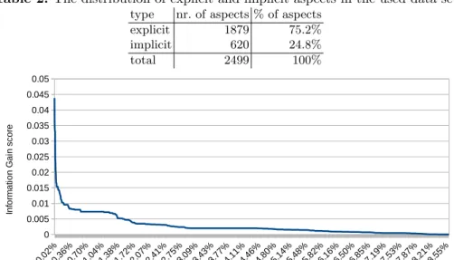
Table 2: The distribution of explicit and implicit aspects in the used data set
type nr. of aspects % of aspects
explicit 1879 75.2%
implicit 620 24.8%
total 2499 100%
Fig. 2:The Information Gain for all features with a non-zero score, in descending order of Information Gain.
words around an aspect should be used to extract features from), and the last part is used for testing. This procedure is repeated ten times, in such a way that the part for testing is different each round. This ensures that each part of the data set has been used for testing exactly once and so a complete evaluation result over the whole data set can be obtained.
From one of the folds, we extracted the list of features and their computed Information Gain. As shown in Fig. 2, the distribution of Information Gain scores over features is highly skewed. Only about 8.6% of the features actually receives a non-zero score.
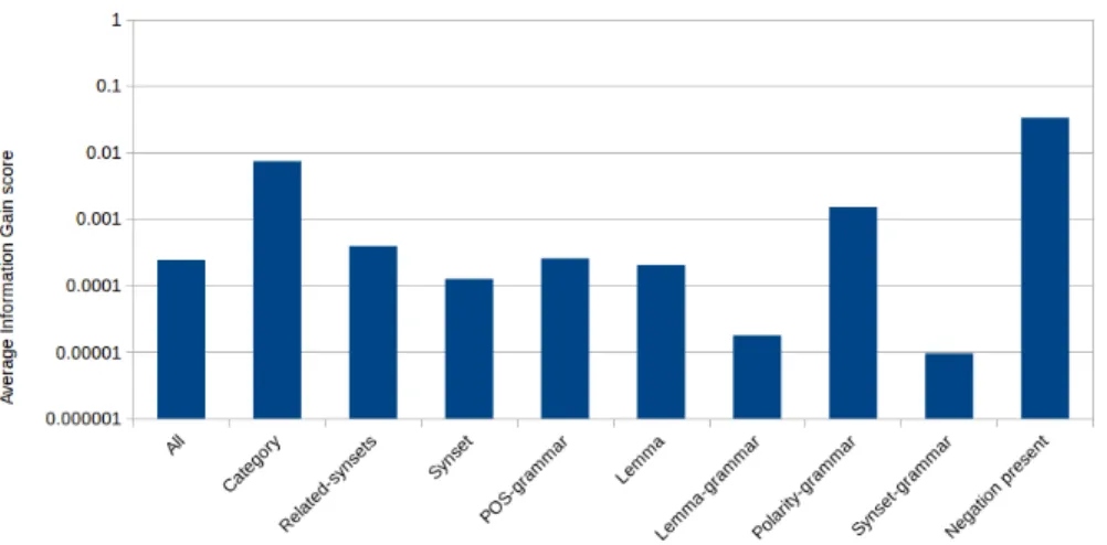
Grouping the features per feature type, we can compute the average Infor-mation Gain for all features of a certain type. This plot, shown in Fig. 3, shows how important, on average, each of the feature types is. Given the fact that the y-axis is logarithmic, the differences between importance are large. Traditional feature types like ‘Negation present’ and ‘Category’ are still crucial to having a good performance, but the new feature type ‘Polarity-grammar’ also shows good performance. The new ‘Related-synsets’ and ‘POS-grammar’ category are in the same league as the traditional ‘Lemma’ category, having an average In-formation Gain. Feature types that are less useful are ‘Lemma-grammar’ and ‘Synset-grammar’, which are very fine-grained and are thus less likely to gener-alize well from training to test data.
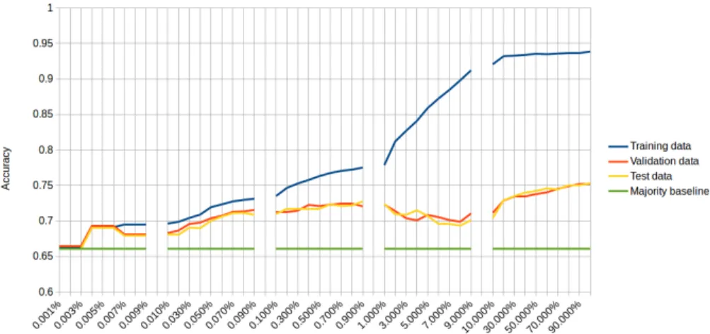
In Fig. 4, the average in-sample accuracy, as well as the accuracy on the validation and test data are presented for a number of values fork, wherekmeans that the topk percent ranked features were used to train and run the SVM. It shows that when using just the top 1% of the features, an accuracy of 72.4% can be obtained, which is only 2.9% less than the performance obtained when using
Fig. 3: The average Information Gain for each feature type.
all features. This point corresponds to a maximum in the performance on the validation data. Other parameters that are optimized using validation data are C, which is on average set to 1, andn, which is on average set to 4. Note that since all parameters that are optimized with validation data are optimized per fold, their exact value differs per fold and thus an average is given. The picture is split into five different levels of granularity on the x-axis, providing more details for lower values ofk. In the first split, the method start at the baseline performance, since at such a low value ofk, no features are selected at all. Then, in the second block, one can see that, because these are all features with high Information Gain, the performance on the test data closely tracks the in-sample performance on the training data. However, in the third split, some minor overfitting starts to occur. The best features have already been used, so lesser features make their way into the SVM, and while in-sample performance goes up, out-of-sample performance does not grow as fast. This effect is illustrated even stronger in the fourth block, where performance on the training data goes up spectacularly, while performance on the test data actually goes down. The features that are added here all have a very low Information Gain.
The last block is slightly different because for almost all of these features, roughly 90% of the total number, the Information Gain is zero. However, as is made evident by the upward slope of the out-of-sample performance, these features are not necessarily useless and the SVM is able to use them to boost performance with a few percent. This is possible due to the fact that, while Information Gain is computed for each feature in isolation, the SVM takes in-teraction effects between features into account. Hence, while these features may not be useful on their own, given the features already available to the SVM, they can still be of use. This interaction effect accounts for the 2.9% penalty to performance increase when using feature selection based on Information Gain.
The diminishing Information Gain is also clearly illustrated in Fig. 5. It follows roughly the same setup in levels of detail as Fig. 4, with this exception
Fig. 4:The average accuracy on training, validation, and test set for each of the subsets of features.
Fig. 5: The average Information Gain score for each of the subsets of added features.
that the first split is combined into the first bar, since not enough features were selected in the first split to create a meaningful set of bars. Furthermore, while Fig. 4 has a cumulative x-axis, this figure does not, showing the average Information Gain of features that are added in each range (instead of all features added up to that point). Given that the lowest 90% of the features has an Information Gain of zero, there are no visible bars in the last split.
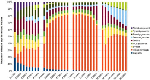
For each of the feature selections, we can also look at how well each type of feature is represented in that subset. Hence, we plot the percentage of features se-lected belonging to each of the feature types in Fig. 6. Features whose proportion decrease when adding more features are generally more important according to the Information Gain ranking, while features whose proportion increases when adding more features are generally less important since they generally have a lower Information Gain. This corresponds to the feature types with high bars in Fig. 3. It is interesting to see that ‘Negation’ and ‘Category’ are small but strong
Fig. 6: Proportion of each feature type for each of the cumulative subsets of features.
feature sets, and that ‘Related-synsets’, while not having many strong features, has many features that get a non-zero Information Gain, making it still a useful category of features.
Analyzing the top ranked features per feature type in Table 3, some of the features are easily recognized as being helpful to detect sentiment. For instance, the lemma ‘not’, as well as its corresponding synset in WordNet are good indi-cators of negative sentiment. Other features, like the ‘SERVICE#GENERAL’ category feature are not so self-evident. These more generic features, while not directly pointing to a certain sentiment value, are still useful by virtue of their statistics. Again looking at the ‘SERVICE#GENERAL’ category, we check the dataset and see that about 56% of all aspects with this category have a negative sentiment, whereas overall, only 30% of the aspects are negative. This is such a sharp deviation from the norm, that having this category label is a strong sign for an aspect to be negative. It seems that in the used data set, people tend to be dissatisfied with the provided service.
Sometimes features that appear in different categories might still represent (almost) the same information. For instance, the two top ‘Lemma-grammar’ features are basically the same as the two top ‘Synset-grammar’ features, corre-sponding to a phrase like “some aspect is ok” or “some aspect is good”. Another example of this is the lemma ‘ok’ and its corresponding synset ‘ok#JJ#1’.
An interesting type of features is the ‘Related-synsets’ category. In Table 3, we seen that any synset that is similar to concepts like ‘big’, ‘alarming’, and ‘satisfactory’ are good predictors of sentiment, and this corresponds well with our intuition. Sometimes, a high ranked feature can give insight into how con-sumers write their reviews. A good example is the ‘CD-dep-$’ feature in the ‘POS-grammar’ category, which denotes a concrete price, such as “$100”, and is
Category Synsets Polarity-grammar
1 SERVICE#GENERAL 3 not#RB#1 6 neutral-amod-positive
40 FOOD#QUALITY 27 ok#JJ#1 7 neutral-amod-neutral
42 RESTAURANT#PRICES 37 good#JJ#1 11 neutral-neg-negative
Related-synsets POS-grammar Lemma-grammar
2 Similar To big#JJ#1 9 NN-amod-JJ 28 ok-cop-be
8 Similar To alarming#JJ#1 25 JJ-cop-VBZ 35 good-cop-be
10 Similar To satisfactory#JJ#1 34 CD-dep-$ 374 good-punct-.
Synset-grammmar Lemma Negation Present
29 ok#JJ#1-cop-be#VB#1 5 not 4 Negation present
45 good#JJ#1-cop-be#VB#1 22 do
705 average#JJ#1-cop-be#VB#1 26 ok
Table 3:Top 3 features for each feature type with their Information Gain based rank.
predominantly used in conjunction with a negative sentiment. Apparently, when people are upset about the price of a restaurant, they feel the need to prove their point by mentioning the exact price.
Last, the ‘Polarity-grammar’ features also score well in terms of Information Gain. The three top features in this category would match phrases such as “good service”, “big portions”, and “not returning”, respectively. Even the ‘neutral-amod-neutral’ is used in a positive context about 80% of the time and is therefore a good predictor of positive sentiment. The first and third feature are obvious predictors for positive and negative sentiment, respectively.
In terms of computing time, if we define the training time when using all features to be 100%, we find that training with 1% of the features takes about 20% of the original time, whereas employing only 0.1% of the features requires just over 1% of the original time.
5
Conclusion and future work
In this paper, filtering individual features using Information Gain is shown to provide good results. With only the 1% best features in terms of Information Gain, an accuracy is obtained that is only 2.9% below the accuracy obtained when using all features. Furthermore, training the SVM with 1% of the features takes only 20% of the time required to train it using all features. Apart from fea-ture selection, we have shown the effectiveness of a number of relatively unknown types of features, such as ‘Related-synsets’ and ‘Polarity-grammar’. For future work, the set of features can be expanded even further to include a comparison of grammar based features against n-gram based features. Also of interest is the context of an aspect from which we compute the sentiment score. Currently, this is determined using a simple word distance around the aspect words, but this could be done in a more advanced way, for instance using grammatical relations or even Rhetorical Structure Theory [9].
Acknowledgments
The authors are supported by the Dutch national program COMMIT. We would like to thank Nienke Dijkstra, Vivian Hinfelaar, Isabelle Houck, Tim van den IJssel, and Eline van de Ven, for many fruitful discussions during this research.
References
1. Baccianella, S., Esuli, A., Sebastiani, F.: SentiWordNet 3.0: An enhanced lexical resource for sentiment analysis and opinion mining. In: Proceedings of the Seventh International Conference on Language Resources and Evaluation (LREC 2010). vol. 10, pp. 2200–2204 (2010)
2. Chang, C., Lin, C.: LIBSVM: A library for support vector machines. ACM Trans-actions on Intelligent Systems and Technology 2(3), 27 (2011)
3. Choi, Y., Cardie, C.: Learning with Compositional Semantics as Structural In-ference for Subsentential Sentiment Analysis. In: Proceedings of the ConIn-ference on Empirical Methods in Natural Language Processing 2008 (EMNLP 2008). pp. 793–801 (2008)
4. Feldman, R.: Techniques and applications for sentiment analysis. Communications of the ACM 56(4), 82–89 (2013)
5. Haddi, E., Liu, X., Shi, Y.: The role of text pre-processing in sentiment analysis. Procedia Computer Science 17, 26 – 32 (2013)
6. Hu, M., Liu, B.: Mining and Summarizing Customer Reviews. In: Proceedings of 10th ACM SIGKDD International Conference on Knowledge Discovery and Data Mining (KDD 2004). pp. 168–177. ACM (2004)
7. Lesk, M.: Automatic sense disambiguation using machine readable dictionaries: How to tell a pine cone from an ice cream cone. In: Proceedings of the Fifth Annual International Conference on Systems Documentation (SIGDOC 1986). pp. 24–26. ACM (1986)
8. Liu, B.: Sentiment Analysis and Opinion Mining. Synthesis Lectures on Human Language Technologies, Morgan & Claypool Publishers (2012)
9. Mann, W.C., Thompson, S.A.: Rhetorical structure theory: Toward a functional theory of text organization. Text-Interdisciplinary Journal for the Study of Dis-course 8(3), 243–281 (1988)
10. Manning, C.D., Surdeanu, M., Bauer, J., Finkel, J., Bethard, S.J., McClosky, D.: The Stanford CoreNLP natural language processing toolkit. In: Proceedings of 52nd Annual Meeting of the Association for Computational Linguistics: System Demonstrations. pp. 55–60. Association for Computational Linguistics (2014) 11. Mitchell, T.M.: Machine Learning. McGraw-Hill, Inc., New York, NY, USA, 1 edn.
(1997)
12. Pontiki, M., Galanis, D., Papageorgiou, H., Manandhar, S., Androutsopoulos, I.: Semeval-2015 task 12: Aspect based sentiment analysis. In: Proceedings of the 9th International Workshop on Semantic Evaluation (SemEval 2015). pp. 486–495. Association for Computational Linguistics (2015)
13. Schouten, K., Frasincar, F.: Survey on aspect-level sentiment analysis. IEEE Trans-actions on Knowledge and Data Engineering 28(3), 813–830 (2016)
14. Titov, I., McDonald, R.: A Joint Model of Text and Aspect Ratings for Sentiment Summarization. In: Proceedings of the 46th Annual Meeting of the Association for Computational Linguistics: Human Language Technologies (HLT 2008). pp. 308–316. ACL (2008)