20 Forecasting. e-text Main Menu Textbook Table of Contents

1009

20

Forecasting

How much will the economy grow over the next year? Where is the stock market headed? What about interest rates? How will consumer tastes be changing? What will be the hot new products?

Forecasters have answers to all these questions. Unfortunately, these answers will more than likely be wrong. Nobody can accurately predict the future every time.

Nevertheless, the future success of any business depends heavily on how savvy its management is in spotting trends and developing appropriate strategies. The leaders of the best companies often seem to have a sixth sense for when to change direction to stay a step ahead of the competition. These companies seldom get into trouble by badly mis-estimating what the demand will be for their products. Many other companies do. The ability to forecast well makes the difference.

The preceding chapter has presented a considerable number of models for the man-agement of inventories. All these models are based on a forecast of future demand for a product, or at least a probability distribution for that demand. Therefore, the missing in-gredient for successfully implementing these inventory models is an approach for fore-casting demand.

Fortunately, when historical sales data are available, some proven statistical fore-casting methods have been developed for using these data to forecast future demand. Such a method assumes that historical trends will continue, so management then needs to make any adjustments to reflect current changes in the marketplace.

Several judgmental forecasting methods that solely use expert judgment also are available. These methods are especially valuable when little or no historical sales data are available or when major changes in the marketplace make these data unreliable for fore-casting purposes.

Forecasting product demand is just one important application of the various forecast-ing methods. A variety of applications are surveyed in the first section. The second section outlines the main judgmental forecasting methods. Section 20.3 then describes time series, which form the basis for the statistical forecasting methods presented in the subsequent five sections. Section 20.9 turns to another important type of statistical forecasting method, regression analysis, where the variable to be forecasted is expressed as a mathematical function of one or more other variables whose values will be known at the time of the fore-cast. The chapter then concludes by surveying forecasting practices in U.S. corporations.

We now will discuss some main areas in which forecasting is widely used. In each case, we will illustrate this use by mentioning one or more actual applications that have been described in published articles. A summary table at the end of the section will tell you where these articles can be found in case you want to read further.

Sales Forecasting

Any company engaged in selling goods needs to forecast the demand for those goods. Manufacturers need to know how much to produce. Wholesalers and retailers need to know how much to stock. Substantially underestimating demand is likely to lead to many lost sales, unhappy customers, and perhaps allowing the competition to gain the upper hand in the marketplace. On the other hand, significantly overestimating demand also is very costly due to (1) excessive inventory costs, (2) forced price reductions, (3) unneeded production or storage capacity, and (4) lost opportunities to market more profitable goods. Successful marketing and production managers understand very well the importance of obtaining good sales forecasts.

TheMerit Brass Companyis a family-owned company that supplies several thousand products to the pipe, valve, and fittings industry. In 1990, Merit Brass embarked on a mod-ernization program that emphasized installing OR methodologies in statistical sales fore-casting and finished-goods inventory management (two activities that go hand in glove). This program led to major improvements in customer service (as measured by product availability) while simultaneously achieving substantial cost reductions.

A major Spanish electric utility,Hidroeléctrica Español, has developed and imple-mented a hierarchy of OR models to assist in managing its system of reservoirs used for generating hydroelectric power. All these models are driven by forecasts of both energy demand (this company’s sales) and reservoir inflows. A sophisticated statistical forecast-ing method is used to forecast energy demand on both a short-term and long-term basis. A hydrological forecasting model generates the forecasts of reservoir inflows.

Airline companies now depend heavily on the high fares paid by business people trav-eling on short notice while providing discount fares to others to help fill the seats. The decision on how to allocate seats to the different fare classes is a crucial one for maxi-mizing revenue. American Airlines,for example, uses statistical forecasting of the demand at each fare to make this decision.

Forecasting the Need for Spare Parts

Although effective sales forecasting is a key for virtually any company, some organiza-tions must rely on other types of forecasts as well. A prime example involves forecasts of the need for spare parts.

Many companies need to maintain an inventory of spare parts to enable them to quickly repair either their own equipment or their products sold or leased to customers. In some cases, this inventory is huge. For example, IBM’s spare-parts inventory described in Sec. 19.8 is valued in the billions of dollars and includes many thousand different parts.

Just as for a finished-goods inventory ready for sale, effective management of a spare-parts inventory depends upon obtaining a reliable forecast of the demand for that

inven-20.1

SOME APPLICATIONS OF FORECASTING

tory. Although the types of costs incurred by misestimating demand are somewhat differ-ent, the consequences may be no less severe for spare parts. For example, the consequence for an airline not having a spare part available on location when needed to continue fly-ing an airplane probably is at least one canceled flight.

To support its operation of several hundred aircraft,American Airlines maintains an extensive inventory of spare parts. Included are over 5,000 different types of rotatable parts (e.g., landing gear and wing flaps) with an average value of $5,000 per item. When a rotatable part on an airplane is found to be defective, it is immediately replaced by a corresponding part in inventory so the airplane can depart. However, the replaced part then is repaired and placed back into inventory for subsequent use as a replacement part.

American Airlines uses a PC-based forecasting system called the Rotatables Alloca-tion and Planning System (RAPS) to forecast demand for the rotatable parts and to help allocate these parts to the various airports. The statistical forecast uses an 18-month his-tory of parts usage and flying hours for the fleet, and then projects ahead based on planned flying hours.

Forecasting Production Yields

The yield of a production process refers to the percentage of the completed items that meet quality standards (perhaps after rework) and so do not need to be discarded. Partic-ularly with high-technology products, the yield frequently is well under 100 percent.

If the forecast for the production yield is somewhat under 100 percent, the size of the production run probably should be somewhat larger than the order quantity to provide a good chance of fulfilling the order with acceptable items. (The difference between the run size and the order quantity is referred to as the reject allowance.) If an expensive setup is required for each production run, or if there is only time for one production run, the reject allowance may need to be quite large. However, an overly large value should be avoided to prevent excessive production costs.

Obtaining a reliable forecast of production yield is essential for choosing an appro-priate value of the reject allowance.

This was the case for the Albuquerque Microelectronics Operation,a dedicated pro-duction source for radiation-hardened microchips. The first phase in the propro-duction of its microchips, the wafer fabrication process, was continuing to provide erratic production yields. For a given product, the yield typically would be quite small (0 to 40 percent) for the first several lots and then would gradually increase to a higher range (35 to 75 per-cent) for later lots. Therefore, a statistical forecasting method that considered this in-creasing trend was used to forecast the production yield.

Forecasting Economic Trends

With the possible exception of sales forecasting, the most extensive forecasting effort is devoted to forecasting economic trends on a regional, national, or even international level. How much will the nation’s gross domestic product grow next quarter? Next year? What is the forecast for the rate of inflation? The unemployment rate? The balance of trade? Statistical models to forecast economic trends (commonly called econometric mod-els) have been developed in a number of governmental agencies, university research cen-ters, large corporations, and consulting firms, both in the United States and elsewhere.

Using historical data to project ahead, these econometric models typically consider a very large number of factors that help drive the economy. Some models include hundreds of variables and equations. However, except for their size and scope, these models resemble some of the statistical forecasting methods used by businesses for sales forecasting, etc. These econometric models can be very influential in determining governmental poli-cies. For example, the forecasts provided by the U.S. Congressional Budget Office strongly guide Congress in developing the federal budgets. These forecasts also help businesses in assessing the general economic outlook.

As an example on a smaller scale, the U.S. Department of Laborcontracted with a consulting firm to develop the unemployment insurance econometric forecasting model (UIEFM). The model is now in use by state employment security agencies around the na-tion. By projecting such fundamental economic factors as unemployment rates, wage lev-els, the size of the labor force covered by unemployment insurance, etc., UIEFM forecasts how much the state will need to pay in unemployment insurance. By projecting tax inflows into the state’s unemployment insurance trust fund, UIEFM also forecasts trust fund bal-ances over a 10-year period. Therefore, UIEFM has proved to be invaluable in managing state unemployment insurance systems and in guiding related legislative policies.

Forecasting Staffing Needs

One of the major trends in the American economy is a shifting emphasis from manufactur-ing to services. More and more of our manufactured goods are bemanufactur-ing produced outside the country (where labor is cheaper) and then imported. At the same time, an increasing num-ber of American business firms are specializing in providing a service of some kind (e.g., travel, tourism, entertainment, legal aid, health services, financial, educational, design, main-tenance, etc.). For such a company, forecasting “sales” becomes forecasting the demand for services, which then translates into forecasting staffing needs to provide those services.

For example, one of the fastest-growing service industries in the United States today is call centers. A call center receives telephone calls from the general public requesting a particular type of service. Depending on the center, the service might be providing tech-nical assistance over the phone, or making a travel reservation, or filling a telephone or-der for goods, or booking services to be performed later, etc. There now are more than 350,000 call centers in the United States, with over $25 billion invested to date and an annual growth rate of 20 percent.

As with any service organization, an erroneous forecast of staffing requirements for a call center has serious consequences. Providing too few agents to answer the telephone leads to unhappy customers, lost calls, and perhaps lost business. Too many agents cause excessive personnel costs.

Section 3.5 described a major OR study that involved personnel scheduling at United Airlines.With over 4,000 reservations sales representatives and support personnel at its 11 reservations offices, and about 1,000 customer service agents at its 10 largest airports, a computerized planning system was developed to design the work schedules for these employees. Although several other OR techniques (including linear programming) were incorporated into this system, statistical forecasting of staffing requirements also was a key ingredient. This system provided annual savings of over $6 million as well as im-proved customer service and reduced support staff requirements.

L.L. Beanis a major retailer of high-quality outdoor goods and apparel. Over 70 per-cent of its total sales volume is generated through orders taken at the company’s call cen-ter. Two 800 numbers are provided, one for placing orders and the second for making in-quiries or reporting problems. Each of the company’s agents is trained to answer just one of the 800 numbers. Therefore, separate statistical forecasting models were developed to forecast staffing requirements for the two 800 numbers on a weekly basis. The improved precision of these models is estimated to have saved L.L. Bean $300,000 annually through enhanced scheduling efficiency.

Other

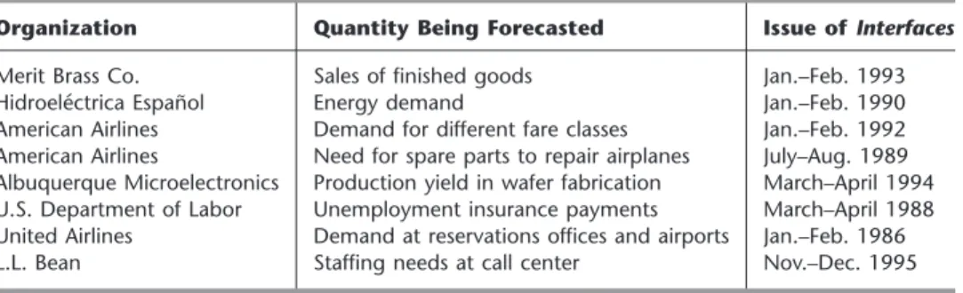
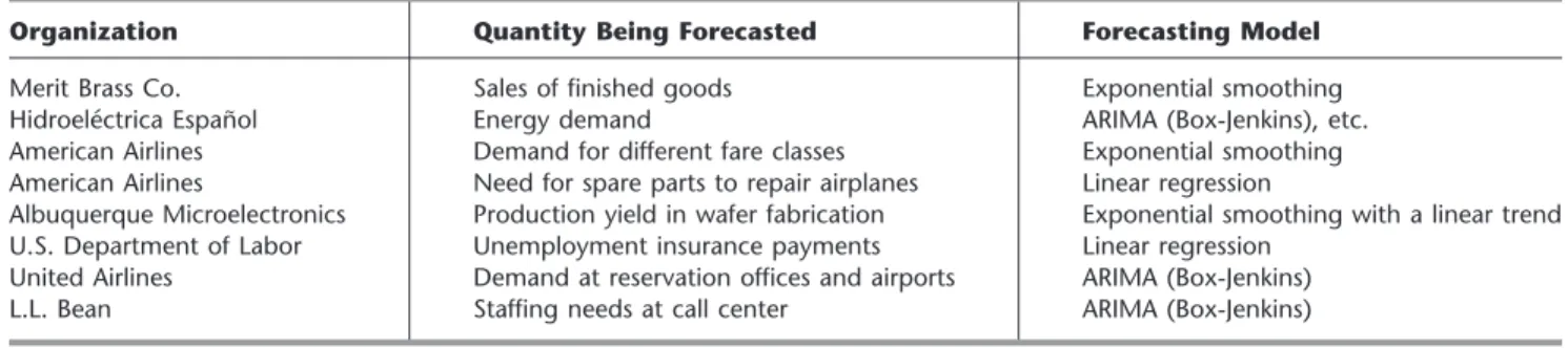
Table 20.1 summarizes the actual applications of statistical forecasting methods presented in this section. The last column cites the issue of Interfaceswhich includes the article that describes each application in detail.

All five categories of forecasting applications discussed in this section use the types of forecasting methods presented in the subsequent sections. There also are other impor-tant categories (including forecasting weather, the stock market, and prospects for new products before market testing) that use specialized techniques that are not discussed here.

20.2 JUDGMENTAL FORECASTING METHODS 1013

TABLE 20.1 Some applications of statistical forecasting methods

Organization Quantity Being Forecasted Issue of Interfaces Merit Brass Co. Sales of finished goods Jan.–Feb. 1993

Hidroeléctrica Español Energy demand Jan.–Feb. 1990

American Airlines Demand for different fare classes Jan.–Feb. 1992 American Airlines Need for spare parts to repair airplanes July–Aug. 1989 Albuquerque Microelectronics Production yield in wafer fabrication March–April 1994 U.S. Department of Labor Unemployment insurance payments March–April 1988 United Airlines Demand at reservations offices and airports Jan.–Feb. 1986 L.L. Bean Staffing needs at call center Nov.–Dec. 1995

Judgmental forecasting methods are, by their very nature, subjective, and they may in-volve such qualities as intuition, expert opinion, and experience. They generally lead to forecasts that are based upon qualitative criteria.

These methods may be used when no data are available for employing a statistical forecasting method. However, even when good data are available, some decision makers prefer a judgmental method instead of a formal statistical method. In many other cases, a combination of the two may be used.

Here is a brief overview of the main judgmental forecasting methods.

1. Manager’s opinion:This is the most informal of the methods, because it simply in-volves a single manager using his or her best judgment to make the forecast. In some cases, some data may be available to help make this judgment. In others, the manager may be drawing solely on experience and an intimate knowledge of the current con-ditions that drive the forecasted quantity.

2. Jury of executive opinion:This method is similar to the first one, except now it in-volves a small group of high-level managers who pool their best judgment to collec-tively make the forecast. This method may be used for more critical forecasts for which several executives share responsibility and can provide different types of expertise.

3. Sales force composite:This method is often used for sales forecasting when a com-pany employs a sales force to help generate sales. It is a bottom-up approachwhereby each salesperson provides an estimate of what sales will be in his or her region. These estimates then are sent up through the corporate chain of command, with managerial review at each level, to be aggregated into a corporate sales forecast.

4. Consumer market survey:This method goes even further than the preceding one in adopting a grass-roots approachto sales forecasting. It involves surveying customers and potential customers regarding their future purchasing plans and how they would respond to various new features in products. This input is particularly helpful for de-signing new products and then in developing the initial forecasts of their sales. It also is helpful for planning a marketing campaign.

5. Delphi method:This method employs a panel of experts in different locations who independently fill out a series of questionnaires. However, the results from each ques-tionnaire are provided with the next one, so each expert then can evaluate this group information in adjusting his or her responses next time. The goal is to reach a rela-tively narrow spread of conclusions from most of the experts. The decision makers then assess this input from the panel of experts to develop the forecast. This involved process normally is used only at the highest levels of a corporation or government to develop long-range forecasts of broad trends.

The decision on whether to use one of these judgmental forecasting methods should be based on an assessment of whether the individuals who would execute the method have the background needed to make an informed judgment. Another factor is whether the ex-pertise of these individuals or the availability of relevant historical data (or a combination of both) appears to provide a better basis for obtaining a reliable forecast.

The next seven sections discuss statistical forecasting methods based on relevant his-torical data.

1_{These times of observation sometimes are actually time periods (months, years, etc.), so we often will refer to} the times as periods.

Most statistical forecasting methods are based on using historical data from a time series. Atime seriesis a series of observations over time of some quantity of interest (a random variable). Thus, if Xiis the random variable of interest at time i, and if observations are taken at times1_{i⫽1, 2, . . . , t, then the observed values}

{X1⫽x1,X2⫽x2, . . . ,Xt⫽xt} are a time series.

For example, the recent monthly sales figures for a product comprises a time series, as il-lustrated in Fig. 20.1.

Because a time series is a description of the past, a logical procedure for forecasting the future is to make use of these historical data. If the past data are indicative of what

20.3

TIME SERIES

we can expect in the future, we can postulate an underlying mathematical model that is representative of the process. The model can then be used to generate forecasts.

In most realistic situations, we do not have complete knowledge of the exact form of the model that generates the time series, so an approximate model must be chosen. Fre-quently, the choice is made by observing the pattern of the time series. Several typical time series patterns are shown in Fig. 20.2. Figure 20.2adisplays a typical time series if the generating process were represented by a constant levelsuperimposed with random fluctuations. Figure 20.2bdisplays a typical time series if the generating process were rep-resented by a linear trend superimposed with random fluctuations. Finally, Fig. 20.2c shows a time series that might be observed if the generating process were represented by a constant level superimposed with a seasonal effecttogether with random fluctuations. There are many other plausible representations, but these three are particularly useful in practice and so are considered in this chapter.

20.3 TIME SERIES 1015 1/99 4/99 2,000 0 4,000 6,000 8,000 10,000

Monthly sales (units sold)

7/99 10/99 1/00 4/00 7/00 FIGURE 20.1

The evolution of the monthly sales of a product illustrates a time series. Time (a) Time (c) Time (b) FIGURE 20.2

Typical time series patterns, with random fluctuations around (a) a constant level, (b) a linear trend, and (c) a constant level plus seasonal effects.

Once the form of the model is chosen, a mathematical representation of the generat-ing process of the time series can be given. For example, suppose that the generatgenerat-ing process is identified as a constant-level modelsuperimposed with random fluctuations, as illustrated in Fig. 20.2a. Such a representation can be given by

Xi⫽A⫹ei, for i⫽1, 2, . . . ,

whereXiis the random variable observed at time i,Ais the constant level of the model,

andei is the random error occurring at time i(assumed to have expected value equal to

zero and constant variance). Let

Ft⫹1⫽forecast of the values of the time series at time t⫹1, given the observed

values,X1⫽x1,X2⫽x2, . . . ,Xt⫽xt.

Because of the random error et⫹1, it is impossible for Ft⫹1to predict the value Xt⫹1⫽ xt⫹1 precisely, but the goal is to have Ft⫹1estimate the constant level A⫽E(Xt⫹1) as

closely as possible. It is reasonable to expect that Ft⫹1will be a function of at least some

of the observed values of the time series.

We now present four alternative forecasting methods for the constant-level model in-troduced in the preceding paragraph. This model, like any other, is only intended to be an idealized representation of the actual situation. For the real time series, at least small shifts in the value of Amay be occurring occasionally. Each of the following methods reflects a different assessment of how recently (if at all) a significant shift may have occurred.

Last-Value Forecasting Method

By interpreting tas the current time,the last-value forecasting procedure uses the value of the time series observed at time t(xt) as the forecast at time t⫹1. Therefore,

Ft⫹1⫽xt.

For example, if xt represents the sales of a particular product in the quarter just ended,

this procedure uses these sales as the forecast of the sales for the next quarter.

This forecasting procedure has the disadvantage of being imprecise; i.e., its variance is large because it is based upon a sample of size 1. It is worth considering only if (1) the underlying assumption about the constant-level model is “shaky”and the process is chang-ing so rapidly that anythchang-ing before time tis almost irrelevant or misleading or (2) the as-sumption that the random error ethas constant variance is unreasonable and the variance

at time tactually is much smaller than at previous times.

The last-value forecasting method sometimes is called the naive method, because statisticians consider it naive to use just a sample size of onewhen additional relevant data are available. However, when conditions are changing rapidly, it may be that the last value is the only relevant data point for forecasting the next value under current conditions. Therefore, decision makers who are anything but naive do occasionally use this method under such circumstances.

Averaging Forecasting Method

This method goes to the other extreme. Rather than using just a sample size of one, this method uses allthe data points in the time series and simply averagesthese points. Thus, the forecast of what the next data point will turn out to be is

Ft⫹1⫽

冱

This estimate is an excellent one if the process is entirely stable, i.e., if the assumptions about the underlying model are correct. However, frequently there exists skepticism about the persistence of the underlying model over an extended time. Conditions inevitably change eventually. Because of a natural reluctance to use very old data, this procedure generally is limited to young processes.

Moving-Average Forecasting Method

Rather than using very old data that may no longer be relevant, this method averages the data for only the last nperiods as the forecast for the next period, i.e.,

Ft⫹1⫽

冱

Note that this forecast is easily updated from period to period. All that is needed each time is to lop off the first observation and add the last one.

Themoving-averageestimator combines the advantages of the last value and

aver-agingestimators in that it uses only recent history and it uses multiple observations. A

disadvantage of this method is that it places as much weight on xt⫺n⫹1as on xt. Intuitively,

one would expect a good method to place more weight on the most recent observation than on older observations that may be less representative of current conditions. Our next method does just this.

Exponential Smoothing Forecasting Method

This method uses the formula

Ft⫹1⫽␣xt⫹(1⫺␣)Ft,

where␣ (0⬍␣⬍1) is called the smoothing constant. (The choice of ␣ is discussed later.) Thus, the forecast is just a weighted sum of the last observation xtand the

preced-ing forecast Ftfor the period just ended. Because of this recursive relationship between Ft⫹1andFt, alternatively Ft⫹1can be expressed as

Ft⫹1⫽␣xt⫹␣(1⫺␣)xt⫺1⫹␣(1⫺␣)2xt⫺2⫹ ⭈⭈⭈.

In this form, it becomes evident that exponential smoothing gives the most weight to xt

and decreasing weights to earlier observations. Furthermore, the first form reveals that the forecast is simple to calculate because the data prior to period tneed not be retained; all that is required is xtand the previous forecast Ft.

Another alternative form for the exponential smoothing technique is given by

Ft⫹1⫽Ft⫹␣(xt⫺Ft),

which gives a heuristic justification for this method. In particular, the forecast of the time series at time t⫹1 is just the preceding forecast at time t plus the productof the fore-casting error at time tand a discount factor ␣. This alternative form is often simpler to use. A measure of effectiveness of exponential smoothing can be obtained under the as-sumption that the process is completely stable, so that X1,X2, . . . are independent,

iden-tically distributed random variables with variance ␴2. It then follows that (for large t) var[Ft⫹1]⬇ᎏ₂ ␣ ⫺ ␴2 ␣ ᎏ ⫽ ᎏ (2⫺ ␴ ␣ 2 )/␣ ᎏ,

so that the variance is statistically equivalent to a moving average with (2⫺␣)/␣ obser-vations. For example, if ␣is chosen equal to 0.1, then (2⫺␣)/␣⫽19. Thus, in terms of its variance, the exponential smoothing method with this value of ␣isequivalent to the moving-average method that uses 19 observations. However, if a change in the process does occur (e.g., if the mean starts increasing), exponential smoothing will react more quickly with better tracking of the change than the moving-average method.

An important drawback of exponential smoothing is that it lags behind a continuing trend; i.e., if the constant-level model is incorrect and the mean is increasing steadily, then the forecast will be several periods behind. However, the procedure can be easily adjusted for trend (and even seasonally adjusted).

Another disadvantage of exponential smoothing is that it is difficult to choose an ap-propriate smoothing constant ␣. Exponential smoothing can be viewed as a statistical filter that inputs raw data from a stochastic process and outputs smoothed estimates of a mean that varies with time. If ␣is chosen to be small, response to change is slow, with resultant smooth estimators. On the other hand, if ␣is chosen to be large, response to change is fast, with re-sultant large variability in the output. Hence, there is a need to compromise, depending upon the degree of stability of the process. It has been suggested that ␣should not exceed 0.3 and that a reasonable choice for ␣is approximately 0.1. This value can be increased temporarily if a change in the process is expected or when one is just starting the forecasting. At the start, a reasonable approach is to choose the forecast for period 2 according to

F2⫽␣x1⫹(1⫺␣)(initial estimate),

where some initial estimate of the constant level Amust be obtained. If past data are avail-able, such an estimate may be the average of these data.

Your OR Courseware includes a pair of Excel templates for each of the four fore-casting methods presented in this section. In each use, one template (without seasonality) applies the method just as described here. The second template (with seasonality) also in-corporates into the method the seasonal factors discussed in the next section.

It is fairly common for a time series to have a seasonal patternwith higher values at cer-tain times of the year than others. For example, this occurs for the sales of a product that is a popular choice for Christmas gifts. Such a time series violates the basic assumption

of a constant-level model,so the forecasting methods presented in the preceding section should not be applied directly.

Fortunately, it is relatively straightforward to make seasonal adjustmentsin such a time series so that these forecasting methods based on a constant-level model can still be applied. We will illustrate the procedure with the following example.

Example. The COMPUTER CLUB WAREHOUSE (commonly referred to as CCW) sells various computer products at bargain prices by taking telephone orders directly from cus-tomers at its call center. Figure 20.3 shows the average number of calls received per day in each of the four quarters of the past three years. Note how the call volume jumps up sharply in each Quarter 4 because of Christmas sales. There also is a tendency for the call volume to be a little higher in Quarter 3 than in Quarter 1 or 2 because of back-to-school sales.

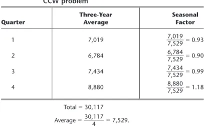
To quantify these seasonal effects, the second column of Table 20.2 shows the average daily call volume for each quarter over the past three years. Underneath this column, the

overall averageover all four quarters is calculated to be 7,529. Dividing the average for

each quarter by this overall average gives the seasonal factorshown in the third column. In general, the seasonal factorfor any period of a year (a quarter, a month, etc.) measures how that period compares to the overall average for an entire year. Specifically, using historical data, the seasonal factor is calculated to be Seasonal factor⫽ .

Your OR Courseware includes an Excel template for calculating these seasonal factors. average for the period

ᎏᎏᎏ overall average

20.5 INCORPORATING SEASONAL EFFECTS INTO FORECASTING METHODS 1019

FIGURE 20.3

The average number of calls received per day at the CCW call center in each of the four quarters of the past three years.

The Seasonally Adjusted Time Series

It is much easier to analyze a time series and detect new trends if the data are first ad-justed to remove the effect of seasonal patterns. To remove the seasonal effects from the time series shown in Fig. 20.3, each of these average daily call volumes needs to be di-vided by the corresponding seasonal factor given in Table 20.2. Thus, the formula is

Seasonally adjusted call volume⫽ ᎏac s t e u a a s l o c n a a l l l f v a o c l t u o m r e ᎏ.

Applying this formula to all 12 call volumes in Fig. 20.3 gives the seasonally adjusted call volumes shown in column Fof the spreadsheet in Fig. 20.4.

In effect, these seasonally adjusted call volumes show what the call volumes would have been if the calls that occur because of the time of the year (Christmas shopping, back-to-school shopping, etc.) had been spread evenly throughout the year instead. Compare the plots in Figs. 20.4 and 20.3. After considering the smaller vertical scale in Fig. 20.4, note how much less fluctuation this figure has than Fig. 20.3 because of removing seasonal ef-fects. However, this figure still is far from completely flat because fluctuations in call vol-ume occur for other reasons beside just seasonal effects. For example, hot new products attract a flurry of calls. A jump also occurs just after the mailing of a catalog. Some ran-dom fluctuations occur without any apparent explanation. Figure 20.4 enables seeing and analyzing these fluctuations in sales volumes that are not caused by seasonal effects.

The General Procedure

After seasonally adjusting a time series, any of the forecasting methods presented in the preceding section (or the next section) can then be applied. Here is an outline of the gen-eral procedure.

1. Use the following formula to seasonally adjust each value in the time series: Seasonally adjusted value⫽ ᎏ

se a a c s t o u n a a l l v f a a l c u t e or ᎏ.

TABLE 20.2 Calculation of the seasonal factors for the CCW problem

Three-Year Seasonal

Quarter Average Factor

1 7,019 ᎏ7 7 , , 0 5 1 2 9 9 ᎏ ⫽0.93 2 6,784 ᎏ6 7 , , 7 5 8 2 4 9 ᎏ ⫽0.90 3 7,434 ᎏ7 7 , , 4 5 3 2 4 9 ᎏ ⫽0.99 4 8,880 ᎏ8 7 , , 8 5 8 2 0 9 ᎏ ⫽1.18 Total⫽30,117 Average⫽ ᎏ30, 4 117 ᎏ ⫽7,529.

2. Select a time series forecasting method.

3. Apply this method to the seasonally adjusted time series to obtain a forecast of the next seasonally adjustedvalue (or values).

4. Multiply this forecast by the corresponding seasonal factor to obtain a forecast of the next actualvalue (without seasonal adjustment).

As mentioned at the end of the preceding section, an Excel template that incorporates seasonal effects is available in your OR Courseware for each of the forecasting methods to assist you with combining the method with this procedure.

20.6 AN EXPONENTIAL SMOOTHING METHOD FOR A LINEAR TREND MODEL 1021

FIGURE 20.4

The seasonally adjusted time series for the CCW problem obtained by dividing each actual average daily call volume in Fig. 20.3 by the corresponding seasonal factor obtained in Table 20.2.

Recall that the constant-level model introduced in Sec. 20.3 assumes that the sequence of random variables {X1,X2, . . . , Xt} generating the time series has a constant expected

value denoted by A, where the goal of the forecast Ft⫹1is to estimate Aas closely as

pos-sible. However, as was illustrated in Fig. 20.2b, some time series violate this assumption by having a continuing trend where the expected values of successive random variables

20.6

AN EXPONENTIAL SMOOTHING METHOD

FOR A LINEAR TREND MODEL

keep changing in the same direction. Therefore, a forecasting method based on the con-stant-level model (perhaps after adjusting for seasonal effects) would do a poor job of forecasting for such a time series because it would be continually lagging behind the trend. We now turn to another model that is designed for this kind of time series.

Suppose that the generating process of the observed time series can be represented by a linear trendsuperimposed with random fluctuations,as illustrated in Fig. 20.2b. De-note the slope of the linear trend by B,where the slope is called the trend factor.The model is represented by

Xi⫽A⫹Bi⫹ei, for i⫽1, 2, . . . ,

whereXiis the random variable that is observed at time i,Ais a constant,Bis the trend

factor, and ei is the random error occurring at time i (assumed to have expected value

equal to zero and constant variance).

For a real time series represented by this model, the assumptions may not be com-pletely satisfied. It is common to have at least small shifts in the values of AandB oc-casionally. It is important to detect these shifts relatively quickly and reflect them in the forecasts. Therefore, practitioners generally prefer a forecasting method that places sub-stantial weight on recent observations and little if any weight on old observations. The exponential smoothing method presented next is designed to provide this kind of approach.

Adapting Exponential Smoothing to This Model

The exponential smoothing method introduced in Sec. 20.4 can be adapted to include the trend factor incorporated into this model. This is done by also using exponential smooth-ing to estimate this trend factor.

Let

Tt⫹1⫽exponential smoothing estimate of the trend factor Bat time t⫹1, given

the observed values,X1⫽x1,X2⫽x2, . . . ,Xt⫽xt.

Given Tt⫹1, the forecast of the value of the time series at time t⫹1 (Ft⫹1) is obtained

simply by adding Tt⫹1to the formula for Ft⫹1given in Sec. 20.4, so

Ft⫹1⫽␣xt⫹(1⫺␣)Ft⫹Tt⫹1.

To motivate the procedure for obtaining Tt⫹1, note that the model assumes that B⫽E(Xi⫹1)⫺E(Xi), for i⫽1, 2, . . . .

Thus, the standard statistical estimator of Bwould be the averageof the observed differ-ences, x2⫺x1, x3⫺x2, . . . ,xt⫺xt⫺1. However, the exponential smoothing approach

recognizes that the parameters of the stochastic process generating the time series (in-cludingAandB) may actually be gradually shifting over time so that the most recent ob-servations are the most reliable ones for estimating the current parameters. Let

Lt⫹1⫽latest trend at time t⫹1 based on the last two values (xtandxt⫺1) and the

last two forecasts (FtandFt⫺1).

The exponential smoothing formula used for Lt⫹1is

ThenTt⫹1is calculated as

Tt⫹1⫽␤Lt⫹1⫹(1⫺␤)Tt,

where␤is the trend smoothing constantwhich, like ␣, must be between 0 and 1. Cal-culating Lt⫹1andTt⫹1in order then permits calculating Ft⫹1with the formula given in

the preceding paragraph.

Getting started with this forecasting method requires making two initial estimates about the status of the time series just prior to beginning forecasting. These initial esti-mates are

x0⫽initial estimate of the expected valueof the time series (A) if the conditions

just prior to beginning forecasting were to remain unchanged without any trend;

T1⫽initial estimate of the trendof the time series (B) just prior to beginning forecasting.

The resulting forecasts for the first two periods are

F1⫽x0⫹T1,

L2⫽␣(x1⫺x0)⫹(1⫺␣)(F1⫺x0),

T2⫽␤L2⫹(1⫺␤)T1,

F2⫽␣x1⫹(1⫺␣)F1⫹T2.

The above formulas for Lt⫹1,Tt⫹1, and Ft⫹1then are used directly to obtain subsequent

forecasts.

Since the calculations involved with this method are relatively involved, a computer commonly is used to implement the method. Your OR Courseware includes two Excel templates (one without seasonal adjustments and one with) for this method.

Application of the Method to the CCW Example

Reconsider the example involving the Computer Club Warehouse (CCW) that was intro-duced in the preceding section. Figure 20.3 shows the time series for this example (rep-resenting the average daily call volume quarterly for 3 years) and then Fig. 20.4 gives the seasonally adjusted time series based on the seasonal factors calculated in Table 20.2. We now will assume that these seasonal factors were determined priorto these three years of data and that the company then was using exponential smoothing with trendto forecast the average daily call volume quarter by quarter over the 3 years based on these data. CCW management has chosen the following initial estimates and smoothing constants:

x0⫽7,500, T1⫽0, ␣⫽0.3, ␤⫽0.3.

Working with the seasonally adjusted call volumes given in Fig. 20.4, these initial es-timates lead to the following seasonally adjusted forecasts.

Y1, Q1: F1⫽7,500⫹0⫽7,500.

Y1, Q2: L2⫽0.3(7,322⫺7,500)⫹0.7(7,500⫺7,500)⫽ ⫺53.4. T2⫽0.3(⫺53.4)⫹0.7(0)⫽ ⫺16.

F2⫽0.3(7,322)⫹0.7(7,500)⫺16⫽7,431.

FIGURE 20.5

The Excel template in your OR Courseware for the exponential smoothing with trend method with seasonal adjustments is applied here to the CCW problem.

20.7 FORECASTING ERRORS 1025

Y1, Q3: L3⫽0.3(7,183⫺7,322)⫹0.7(7,431⫺7,500)⫽ ⫺90. T3⫽0.3(⫺90)⫹0.7(⫺16)⫽ ⫺38.2.

F3⫽0.3(7,183)⫹0.7(7,431)⫺38.2⫽7,318. ⯗

The Excel template in Fig. 20.5 shows the results from these calculations for all 12 quar-ters over the 3 years, as well as for the upcoming quarter. The middle of the figure shows the plots of all the seasonally adjusted call volumes and seasonally adjusted forecasts. Note how each trend up or down in the call volumes causes the forecasts to gradually trend in the same direction, but then the trend in the forecasts takes a couple of quarters to turn around when the trend in call volumes suddenly reverses direction. Each number in column I is calculated by multiplying the seasonally adjusted forecast in column H by the corresponding seasonal factor in column M to obtain the forecast of the actual value (not seasonally adjusted) for the average daily call volume. Column J then shows the re-sultingforecasting errors(the absolute value of the difference between columns D and I).

Forecasting More Than One Time Period Ahead

We have focused thus far on forecasting what will happen in the nexttime period (the next quarter in the case of CCW). However, decision makers sometimes need to forecast further into the future. How can the various forecasting methods be adapted to do this? In the case of the methods for a constant-level model presented in Sec. 20.4, the fore-cast for the next period Ft⫹1also is the best available forecast for subsequent periods as

well. However, when there is a trendin the data, as we are assuming in this section, it is important to take this trend into account for long-range forecasts. Exponential smoothing

with trendprovides a straightforward way of doing this. In particular, after determining

theestimated trend Tt⫹1, this method’s forecast for ntime periods into the future is

Ft⫹n⫽␣xt⫹(1⫺␣)Ft⫹nTt⫹1.

Several forecasting methods now have been presented. How does one choose the appro-priate method for any particular application? Identifying the underlying model that best fits the time series (constant-level, linear trend, etc., perhaps in combination with seasonal effects) is an important first step. Assessing how stablethe parameters of the model are, and so how much reliance can be placed on older data for forecasting, also helps to nar-row down the selection of the method. However, the final choice between two or three methods may still not be clear. Some measure of performance is needed.

The goal is to generate forecasts that are as accurate as possible, so it is natural to base a measure of performance on the forecasting errors.

Theforecasting error(also called the residual) for any period tis the absolute value of the deviation of the forecast for period t(Ft) from what then turns out to be the observed

value of the time series for period t(xt). Thus, letting Etdenote this error, Et⫽xt⫺Ft.

For example, column J of the spreadsheet in Fig. 20.5 gives the forecasting errors when applyingexponential smoothing with trendto the CCW example.

Given the forecasting errors for ntime periods (t⫽1, 2, . . . ,n), two popular mea-sures of performance are available. One, called the mean absolute deviation (MAD)is simply the average of the errors, so

MAD⫽ .

This is the measure shown in cell M31 of Fig. 20.5. (Most of the Excel templates for this chapter use this measure.) The other measure, called the mean square error (MSE), in-stead averages the squareof the forecasting errors, so

MSE⫽ .

The advantages of MAD are its ease of calculation and its straightforward interpre-tation. However, the advantage of MSE is that it imposes a relatively large penalty for a large forecasting error that can have serious consequences for the organization while al-most ignoring inconsequentially small forecasting errors. In practice, managers often pre-fer to use MAD, whereas statisticians generally prepre-fer MSE.

Either measure of performance might be used in two different ways. One is to com-pare alternative forecasting methods in order to choose one with which to begin fore-casting. This is done by applying the methods retrospectivelyto the time series in the past (assuming such data exist). This is a very useful approach as long as the future behavior of the time series is expected to resemble its past behavior. Similarly, this retrospective testing can be used to help select the parameters for a particular forecasting method, e.g., the smoothing constant(s) for exponential smoothing. Second, after the real forecasting begins with some method, one of the measures of performance (or possibly both) nor-mally would be calculated periodically to monitor how well the method is performing. If the performance is disappointing, the same measure of performance can be calculated for alternative forecasting methods to see if any of them would have performed better.

冱

冱

In practice, a forecasting method often is chosen without adequately checking whether the underlying model is an appropriate one for the application. The beauty of the Box-Jenk-ins methodis that it carefully coordinates the model and the procedure. (Practitioners of-ten use this name for the method because it was developed by G.E.P. Box and G.M. Jenk-ins. An alternative name is the ARIMA method, which is an acronym for autoregressive integrated moving average.) This method employs a systematic approach to identifying an appropriate model, chosen from a rich class of models. The historical data are used to test the validity of the model. The model also generates an appropriate forecasting procedure. To accomplish all this, the Box-Jenkins method requires a great amount of past data (a minimum of 50 time periods), so it is used only for major applications. It also is a so-phisticated and complex technique, so we will provide only a conceptual overview of the method. (See Selected References 2 and 6 for further details.)

The Box-Jenkins method is iterative in nature. First, a model is chosen. To choose this model, we must compute autocorrelations and partial autocorrelations and examine their patterns. An autocorrelationmeasures the correlation between time series values sep-arated by a fixed number of periods. This fixed number of periods is called the lag. There-fore, the autocorrelation for a lag of two periods measures the correlation between every other observation; i.e., it is the correlation between the original time series and the same series moved forward two periods. The partial autocorrelationis a conditional autocor-relation between the original time series and the same series moved forward a fixed num-ber of periods, holding the effect of the other lagged times fixed. Good estimates of both the autocorrelations and the partial autocorrelations for all lags can be obtained by using a computer to calculate the sample autocorrelations and the sample partial autocorrela-tions. (These are “good”estimates because we are assuming large amounts of data.)

From the autocorrelations and the partial autocorrelations, we can identify the functional form of one or more possible models because a rich class of models is characterized by these quantities. Next we must estimate the parameters associated with the model by using the his-torical data. Then we can compute the residuals (the forecasting errors when the forecasting is done retrospectively with the historical data) and examine their behavior. Similarly, we can examine the behavior of the estimated parameters. If both the residuals and the estimated pa-rameters behave as expected under the presumed model, the model appears to be validated. If they do not, then the model should be modified and the procedure repeated until a model is validated. At this point, we can obtain an actual forecast for the next period.

For example, suppose that the sample autocorrelations and the sample partial auto-correlations have the patterns shown in Fig. 20.6. The sample autoauto-correlations appear to decrease exponentially as a function of the time lags, while the same partial autocorrela-tions have spikes at the first and second time lags followed by values that seem to be of negligible magnitude. This behavior is characteristic of the functional form

Xt⫽B0⫹B1Xt⫺1⫹B2Xt⫺2⫹et.

Assuming this functional form, we use the time series data to estimate B0,B1, and B2.

Denote these estimates by b0,b1, and b2, respectively. Together with the time series data,

we then obtain the residuals

xt⫺(b0⫹b1xt⫺1⫹b2xt⫺2). 20.8 BOX-JENKINS METHOD 1027 Sample autocorrelation 0 1 2 3 4 5 6 Time lags

Sample partial autocorrelation

0 1 2 3 4 5 6 Time lags FIGURE 20.6

Plot of sample autocorrelation and partial autocorrelation versus time lags.

If the assumed functional form is adequate, the residuals and the estimated parameters should behave in a predictable manner. In particular, the sample residuals should behave approximately as independent, normally distributed random variables, each having mean 0 and variance ␴2(assuming that et, the random error at time period t, has mean 0 and

variance ␴2). The estimated parameters should be uncorrelated and significantly different from zero. Statistical tests are available for this diagnostic checking.

The Box-Jenkins procedure appears to be a complex one, and it is. Fortunately, com-puter software is available. The programs calculate the sample autocorrelations and the sample partial autocorrelations necessary for identifying the form of the model. They also estimate the parameters of the model and do the diagnostic checking. These programs, how-ever, cannot accurately identify one or more models that are compatible with the autocor-relations and the partial autocorautocor-relations. Expert human judgment is required. This exper-tise can be acquired, but it is beyond the scope of this text. Although the Box-Jenkins method is complicated, the resulting forecasts are extremely accurate and, when the time horizon is short, better than most other forecasting methods. Furthermore, the procedure produces a measure of the forecasting error.

In the preceding six sections, we have focused on time series forecasting methods,i.e., methods that forecast the next value in a time series based on its previous values. We now turn to another type of approach to forecasting.

Causal Forecasting

In some cases, the variable to be forecasted has a rather direct relationship with one or more other variables whose values will be known at the time of the forecast. If so, it would make sense to base the forecast on this relationship. This kind of approach is called causal forecasting.

Causal forecastingobtains a forecast of the quantity of interest (the dependent variable) by relating it directly to one or more other quantities (the independentvariables) that drive the quantity of interest.

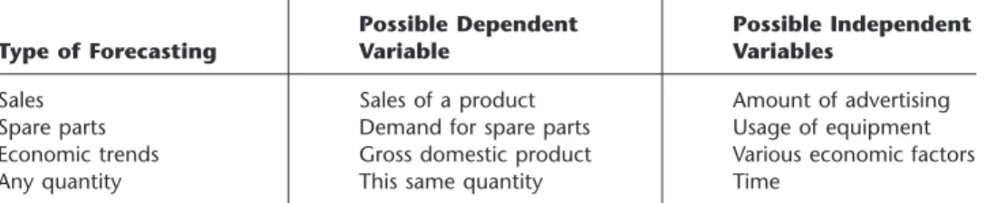
Table 20.3 shows some examples of the kinds of situations where causal forecasting sometimes is used. In each of the first three cases, the indicated dependent variable can be expected to go up or down rather directly with the independent variable(s) listed in the rightmost column. The last case also applies when some quantity of interest (e.g., sales

20.9

CAUSAL FORECASTING WITH LINEAR REGRESSION

TABLE 20.3 Possible examples of causal forecasting

Possible Dependent Possible Independent

Type of Forecasting Variable Variables

Sales Sales of a product Amount of advertising

Spare parts Demand for spare parts Usage of equipment

Economic trends Gross domestic product Various economic factors

of a product) tends to follow a steady trend upward (or downward) with the passage of time (the independent variable that drives the quantity of interest).

As one specific example, Sec. 20.1 includes a description of American Airline’s elab-orate system for forecasting its need for expensive spare parts (its “rotatable” parts) to continue operating its fleet of several hundred airplanes. This system uses causal fore-casting, where the demand for spare parts is the dependent variable and the number of flying hours is the independent variable. This makes sense because the demand for spare parts should be roughly proportional to the number of flying hours for the fleet.

Linear Regression

We will focus on the type of causal forecasting where the mathematical relationship between the dependent variable and the independent variable(s) is assumed to be a linear one (plus some random fluctuations). The analysis in this case is referred to as linear regression.

To illustrate the linear regression approach, suppose that a publisher of textbooks is concerned about the initial press run for her books. She sells books both through book-stores and through mail orders. This latter method uses an extensive advertising campaign on line, as well as through publishing media and direct mail. The advertising campaign is conducted prior to the publication of the book. The sales manager has noted that there is a rather interesting linear relationship between the number of mail orders and the num-ber sold through bookstores during the first year. He suggests that this relationship be ex-ploited to determine the initial press run for subsequent books.

Thus, if the number of mail order sales for a book is denoted by Xand the number of bookstore sales by Y, then the random variables XandY exhibit a degree of

associa-tion. However there is no functional relationship between these two random variables;

i.e., given the number of mail order sales, one does not expect to determine exactly the number of bookstore sales. For any given number of mail order sales, there is a range of possible bookstore sales, and vice versa.

What, then, is meant by the statement,“The sales manager has noted that there is a rather interesting linear relationship between the number of mail orders and the number sold through bookstores during the first year”? Such a statement implies that the expected

valueof the number of bookstore sales is linear with respect to the number of mail order

sales, i.e.,

E[YX⫽x]⫽A⫹Bx.

Thus, if the number of mail order sales is xfor many different books, the average num-ber of corresponding bookstore sales would tend to be approximately A⫹Bx. This rela-tionship between XandYis referred to as a degree of association model.

As already suggested in Table 20.3, other examples of this degree of association model can easily be found. A college admissions officer may be interested in the relationship be-tween a student’s performance on the college entrance examination and subsequent per-formance in college. An engineer may be interested in the relationship between tensile strength and hardness of a material. An economist may wish to predict a measure of in-flation as a function of the cost of living index, and so on.

The degree of association model is not the only model of interest. In some cases, there exists a functional relationshipbetween two variables that may be linked linearly.

In a forecasting context, one of the two variables is time, while the other is the variable of interest. In Sec. 20.6, such an example was mentioned in the context of the generating process of the time series being represented by a linear trend superimposed with random fluctuations, i.e.,

Xt⫽A⫹Bt⫹et,

whereAis a constant,Bis the slope, and etis the random error, assumed to have expected

value equal to zero and constant variance. (The symbol Xtcan also be read as Xgiven tor

asXt.) It follows that

E(Xt)⫽A⫹Bt.

Note that both the degree of association model and the exact functional relationship

model lead to the same linear relationship, and their subsequent treatment is almost iden-tical. Hence, the publishing example will be explored further to illustrate how to treat both kinds of models, although the special structure of the model

E(Xt)⫽A⫹Bt,

withttaking on integer values starting with 1, leads to certain simplified expressions. In the standard notation of regression analysis,Xrepresents the independent variableand

Yrepresents the dependent variableof interest. Consequently, the notational expression for this special time series model now becomes

Yt⫽A⫹Bt⫹et.

Method of Least Squares

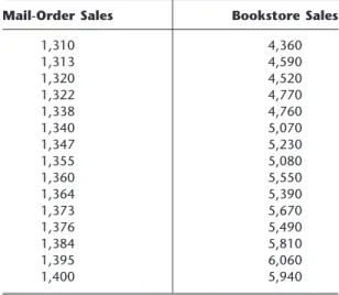
Suppose that bookstore sales and mail order sales are given for 15 books. These data ap-pear in Table 20.4, and the resulting plot is given in Fig. 20.7.

TABLE 20.4 Data for the mail-order and bookstore sales example

Mail-Order Sales Bookstore Sales

1,310 4,360 1,313 4,590 1,320 4,520 1,322 4,770 1,338 4,760 1,340 5,070 1,347 5,230 1,355 5,080 1,360 5,550 1,364 5,390 1,373 5,670 1,376 5,490 1,384 5,810 1,395 6,060 1,400 5,940

It is evident that the points in Fig. 20.7 do not lie on a straight line. Hence, it is not clear where the line should be drawn to show the linear relationship. Suppose that an ar-bitrary line, given by the expression y~⫽a⫹bx, is drawn through the data. A measure of how well this line fits the data can be obtained by computing the sum of squaresof the vertical deviations of the actual points from the fitted line. Thus, let yirepresent the

book-store sales of the ith book and xi the corresponding mail order sales. Denote by y~i the

point on the fitted line corresponding to the mail order sales of xi. The proposed measure

of fit is then given by

Q⫽(y1⫺~y1)2⫹(y2⫺~y2)2⫹ ⭈⭈⭈ ⫹(y15⫺y~15)2⫽

冱

20.9 CAUSAL FORECASTING WITH LINEAR REGRESSION 1031

6,000 5,900 5,800 5,700 5,600 5,500 5,400 5,300 5,200 5,100 5,000 4,900 4,800 4,700 4,600 4,500 4,400 4,300 1,300 1,320 1,340 1,360 1,380 1,400 Mail order sales

Bookstore sales

FIGURE 20.7

Plot of mail order sales versus bookstore sales from Table 20.3.

The usual method for identifying the “best”fitted line is the method of least squares. This method chooses that line a⫹bx that makes Qa minimum. Thus, a andbare ob-tained simply by setting the partial derivatives of Qwith respect to aandbequal to zero and solving the resulting equations. This method yields the solution

b⫽ ⫽ and a⫽y_苶⫺bx_苶, where x 苶⫽

冱

冱

(Note that y_苶is not the same as y~⫽a⫹bxdiscussed in the preceding paragraph.) For the publishing example, the data in Table 20.4 and Fig. 20.7 yield

x 苶⫽1,353.1, y 苶⫽5,219.3,

冱

冱

Hence, the least-squares estimate of bookstore sales y~ with mail order sales xis given by

y

~_{⫽ ⫺19,041.9⫹17.930x,}

and this is the line drawn in Fig. 20.7. Such a line is referred to as a regression line. An Excel template called Linear Regression is available in your OR Courseware for calculating a regression line in this way.

This regression line is useful for forecasting purposes. For a given value of x, the cor-responding value of yrepresents the forecast.

The decision maker may be interested in some measure of uncertainty that is sociated with this forecast. This measure is easily obtained provided that certain

as-冱

冢

冱

冱

冣

冫

冱

冢

冱

冣

冫

冱

冱

sumptions can be made. Therefore, for the remainder of this section, it is assumed that

1. A random sample of npairs (x1,Y1), (x2,Y2), . . . , (xn,Yn) is to be taken.

2. TheYiare normally distributed with mean A⫹Bxiand variance ␴2(independent of i).

The assumption that Yiis normally distributed is not a critical assumption in

deter-mining the uncertainty in the forecast, but the assumption of constant variance is crucial. Furthermore, an estimate of this variance is required.

An unbiased estimate of ␴2is given bysy2x, where

sy 2 x⫽

冱

Confidence Interval Estimation of E(Yxⴝx*)

A very important reason for obtaining the linear relationship between two variables is to use the line for future decision making. From the regression line, it is possible to estimate

E(Yx) by a pointestimate (the forecast) and a confidence intervalestimate (a measure of forecast uncertainty).

For example, the publisher might want to use this approach to estimate the expected number of bookstore sales corresponding to mail order sales of, say, 1,400, by both a point estimate and a confidence interval estimate for forecasting purposes.

A point estimate of E(Yx⫽x*) is given by

y

~*⫽a⫹bx*,

wherex* denotes the given value of the independent variable and y~* is the corresponding

point estimate.

The endpoints of a (100)(1⫺␣) percent confidence interval for E(Yx⫽x*) are given by a⫹bx*⫺t␣/2;n⫺2syx

冪

莦莦

冪

莦莦

wheresy2xis the estimate of ␴2, and t␣/2;n⫺2is the 100␣/2 percentage point of the t

dis-tribution with n⫺2 degrees of freedom (seeTable A5.2 of Appendix 5). Note that the in-terval is narrowest where x*⫽x_苶, and it becomes wider as x* departs from the mean.

In the publishing example with x*⫽1,400,sy2xis computed from the data in Table

20.4 to be 17,030, so syx⫽130.5. If a 95 percent confidence interval is required, Table

A5.2 gives t0.025;13⫽2.160. The earlier calculation of a andbyields a⫹bx*⫽ ⫺19,041.9⫹17.930(1,400)⫽6,060 (x*⫺x_苶)2 ᎏᎏ

冱

冱

as the point estimate of E(Y1,400), that is, the forecast. Consequentially, the confidence limits corresponding to mail order sales of 1,400 are

Lower confidence limit⫽6,060⫺2.160(130.5)

冪

莦

莦

Upper confidence limit⫽6,060⫹2.160(130.5)

冪

莦

莦

The fact that the confidence interval was obtained at a data point (x⫽1,400) is purely coincidental.

The Excel template for linear regression in your OR Courseware does most of the computational work involved in calculating these confidence limits. In addition to com-putingaandb(the regression line), it calculates sy

2 x,x苶, and

冱

The confidence interval statement for the expected number of bookstore sales corre-sponding to mail order sales of 1,400 may be useful for budgeting purposes, but it is not too useful for making decisions about the actualpress run. Instead of obtaining bounds on the expectednumber of bookstore sales, this kind of decision requires bounds on what

the actual bookstore sales will be, i.e., a prediction intervalon the value that the

ran-dom variable (bookstore sales) takes on. This measure is a differentmeasure of forecast uncertainty.

The two endpoints of a prediction interval are given by the expressions

a⫹bx⫹⫺t␣/2;n⫺2syx

冪

莦

莦莦

冪

莦

莦莦

For any given value of x(denoted here by x⫹), the probability is 1⫺␣that the value of the future Y⫹associated with x⫹will fall in this interval.

Thus, in the publishing example, if x⫹is 1,400, then the corresponding 95 percent prediction interval for the number of bookstore sales is given by 6,060⫾315, which is naturally wider than the confidence interval for the expected number of bookstore sales, 6,060⫾141.

This method of finding a prediction interval works fine if it is only being done once. However, it is not feasible to use the same data to find multiple prediction intervals with various values of x⫹in this way and then specify a probability that allthese predictions will be correct. For example, suppose that the publisher wants prediction intervals for

sev-(x_⫹⫺x_苶)2 ᎏᎏ

冱

冱

eral different books. For each individual book, she still is able to use these expressions to find the prediction interval and then make the prediction that the bookstore sales will be within this interval, where the probability is 1⫺␣ that the prediction will be correct. However, what she cannot do is specify a probability that allthese predictions will be cor-rect. The reason is that these predictions are all based upon the same statistical data, so the predictions are not statistically independent. Ifthe predictions were independent and if kfuture bookstore sales were being predicted, with each prediction being made with probability 1⫺␣, then the probability would be (1⫺␣)k_{thatall kpredictions of future}

bookstore sales will be correct. Unfortunately, the predictions are notindependent, so the actual probability cannot be calculated, and (1⫺␣)k_{does not even provide a reasonable}

approximation.

This difficulty can be overcome by using simultaneous tolerance intervals.Using this technique, the publisher can take the mail order sales of any book, find an interval (based on the previously determined linear regression line) that will contain the actual bookstore sales with probability at least 1⫺␣, and repeat this for any number of books having the same or different mail order sales. Furthermore, the probability is Pthat all

these predictions will be correct. An alternative interpretation is as follows. If every pub-lisher followed this procedure, each using his or her own linear regression line, then 100P

percent of the publishers (on average) would find that at least 100(1⫺␣) percent of their bookstore sales fell into the predicted intervals. The expression for the endpoints of each such tolerance interval is given by

a⫹bx⫹⫺c**syx

冪

莦莦

冪

莦莦

wherec** is given in Table 20.5.

Thus, the publisher can predict that the bookstore sales corresponding to known mail order sales will fall in these tolerance intervals. Such statements can be made for as many books as the publisher desires. Furthermore, the probability is Pthat at least 100(1⫺␣) percent of bookstore sales corresponding to mail order sales will fall in these intervals. If

Pis chosen as 0.90 and ␣⫽0.05, the appropriate value of c** is 11.625. Hence, the num-ber of bookstore sales corresponding to mail order sales of 1,400 books is predicted to fall in the interval 6,060⫾759. If another book had mail order sales of 1,353, the book-store sales are predicted to fall in the interval 5,258⫾390, and so on. At least 95 percent of the bookstore sales will fall into their predicted intervals, and these statements are made with confidence 0.90.

To summarize, we now have described three measures of forecast uncertainty. The first (in the preceding subsection) is a confidence interval on the expected value of the random variable Y(for example, bookstore sales) given the observed value xof the inde-pendent variable X(for example, mail order sales). The second is a prediction intervalon

(x⫹⫺x苶) 2 ᎏᎏ

冱

冱

theactual valuethatYwill take on, given x. The third is simul