Nova Southeastern University
NSUWorks
CEC Theses and Dissertations College of Engineering and Computing
2018
Wireless Sensor Network Clustering with Machine
Learning
Larry Townsend
Nova Southeastern University,[email protected]
This document is a product of extensive research conducted at the Nova Southeastern UniversityCollege of Engineering and Computing. For more information on research and degree programs at the NSU College of Engineering and Computing, please clickhere.
Follow this and additional works at:https://nsuworks.nova.edu/gscis_etd Part of theComputer Sciences Commons
Share Feedback About This Item
This Dissertation is brought to you by the College of Engineering and Computing at NSUWorks. It has been accepted for inclusion in CEC Theses and Dissertations by an authorized administrator of NSUWorks. For more information, please [email protected].
NSUWorks Citation
Larry Townsend. 2018.Wireless Sensor Network Clustering with Machine Learning.Doctoral dissertation. Nova Southeastern University. Retrieved from NSUWorks, College of Engineering and Computing. (1042)
Wireless Sensor Network Clustering with Machine Learning
by Larry Townsend
A dissertation submitted in partial fulfillment of the requirements for the degree of Doctor of Philosophy
in
Computer Science
College of Engineering and Computing Nova Southeastern University
ii
An Abstract of a Dissertation Submitted to Nova Southeastern University in Partial Fulfillment of the Requirements for the Degree of Doctor of Philosophy
Wireless Sensor Network Clustering with Machine Learning by
Larry Townsend August 2018
Wireless sensor networks (WSNs) are useful in situations where a low-cost network needs to be set up quickly and no fixed network infrastructure exists. Typical applications are for military exercises and emergency rescue operations. Due to the nature of a wireless network, there is no fixed routing or intrusion detection and these tasks must be done by the individual network nodes. The nodes of a WSN are mobile devices and rely on battery power to function. Due the limited power resources available to the devices and the tasks each node must perform, methods to decrease the overall power consumption of WSN nodes are an active research area.
This research investigated using genetic algorithms and graph algorithms to determine a clustering arrangement of wireless nodes that would reduce WSN power consumption and thereby prolong the lifetime of the network. The WSN nodes were partitioned into clusters and a node elected from each cluster to act as a cluster head. The cluster head managed routing tasks for the cluster, thereby reducing the overall WSN power usage. The clustering configuration was determined via genetic algorithm and graph algorithms.
The fitness function for the genetic algorithm was based on the energy used by the nodes. It was found that the genetic algorithm was able to cluster the nodes in a near-optimal
configuration for energy efficiency. Chromosome repair was also developed and implemented. Two different repair methods were found to be successful in producing near-optimal solutions and reducing the time to reach the solution versus a standard genetic algorithm. It was also found the repair methods were able to implement gateway nodes and energy balance to further reduce network energy consumption.
iii
We hereby certify that this dissertation, submitted by Larry Townsend, conforms to acceptable standards and is fully adequate in scope and quality to fulfill the dissertation requirements for the degree of Doctor of Philosophy.
College of Engineering and Computing Nova Southeastern University
1 Table of Contents Abstract ii Chapters Table of Contents ... 1 List of Figures ... 3 List of Tables ... 5 Introduction ... 6 Background ... 6 Problem Statement ... 13 Formal Definition ... 14 Dissertation Goal ... 17 Research Questions ... 18
Relevance and Significance ... 19
Barriers and Issues ... 20
Assumptions, Limitations and Delimitations ... 21
Assumptions. ... 21
Limitations. ... 22
Delimitations. ... 22
Summary ... 23
Review of the Literature ... 25
P-median ... 25
Wireless sensor networks and MANETs ... 35
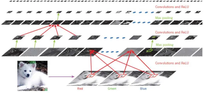
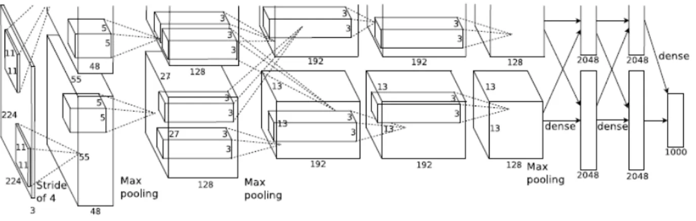
Deep Learning ... 46
Summary ... 51
Methodology ... 52
Overview ... 52
Chromosome Encoding ... 53
2 Helper Functions ... 58 Specific Methods ... 58 Phase 1. ... 59 Phase 2. ... 62 Phase 3. ... 68 Phase 4. ... 70 Phase 5. ... 72 Data set ... 73 Resources ... 73 Summary ... 73 Results ... 75 Overview ... 75 Phase 1. ... 75 Phase 2. ... 86 Phase 3.. ... 108 Phase 4. ... 113 Phase 5. ... 123
Conclusions, Implications, Recommendations, and Summary ... 128
Conclusions ... 128 Implications ... 130 Recommendations ... 131 Summary ... 132 References ... 139 Appendix A ... 142 List of Symbols ... 142 Appendix B ... 145
3
List of Figures
Figure 1. WSN (Akyildiz et al., 2002) ... 7
Figure 2. WSN (Abbasi & Younis, 2007)... 7
Figure 3. WSN (Younis, Krunz & Ramasubramani) ... 8
Figure 4. Disjoint Groups (Domínguez & Muñoz, 2008) ... 34
Figure 5. Clusters (Rousseeuw, 1987) ... 38
Figure 6. ConvNet (LeCun, Bengio & Hinton, 2015) ... 48
Figure 7. ConvNet (Krizhevsky, Sutskever & Hinton, 2012)... 50
Figure 8. Typical chromosome ... 53
Figure 9. 6-Node WSN ... 54
Figure 10. WSN with gateway node ... 70
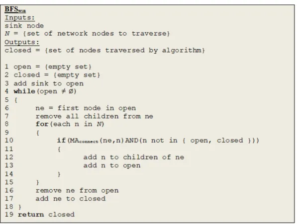
Figure 11. Algorithm BFSwsn ... 80
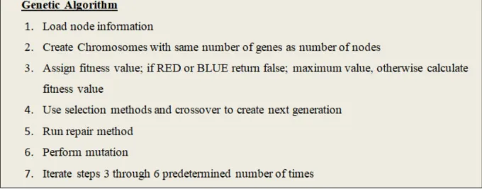
Figure 12. Genetic Algorithm ... 82
Figure 13. 6-Node Network ... 83
Figure 14. 8-Node Network ... 83
Figure 15. Optimal Configuration... 84
Figure 16. Optimal Configuration... 85
Figure 17. 44-Node Network ... 86
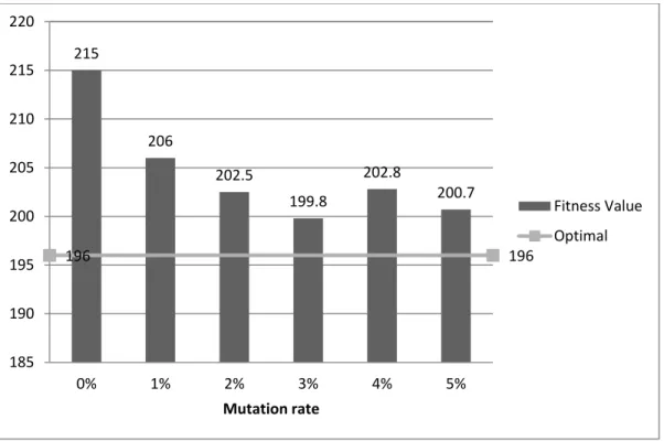
Figure 18. Mutation Results - Fitness ... 92
Figure 19. Mutation Results - Iterations ... 92
Figure 20. Genetic Algorithm ... 93
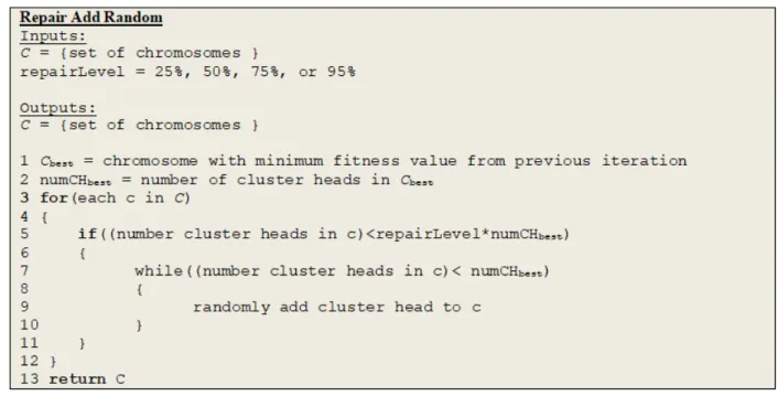
Figure 21. Add Random ... 94
4
Figure 23. Algorithm ARrepair... 100
Figure 24. Timing Results ... 101
Figure 25. Algorithm BFSsep ... 103
Figure 26. Algorithm BFSrand ... 105
Figure 27. BFSrepair ... 106
Figure 28. Timing Comparison ... 107
Figure 29. Energy Calculation ... 109
Figure 30. Algorithm ARrepair with Gateway Nodes ... 115
Figure 31. Algorithm BFSrepair with Gateway Nodes ... 116
Figure 32. Network Creator ... 118
Figure 33. 100-Node Network ... 119
Figure 34. Sparse 100-Node Network ... 121
Figure 35. Algorithm BFSrepair with Energy Balance ... 124
Figure 36. Results, 44-Node Network ... 125
5 List of Tables
Table 1. 6-node network ... 76
Table 2. Selection Methods Results ... 90
Table 3. Output ... 90
Table 4. Results Random Add ... 95
Table 5. Results Add CH ... 96
Table 6. Results ARrepair ... 100
Table 7. Results Repair Comparison ... 106
Table 8. WSN Nodes with Rounds ... 108
Table 9. Varying Message Percentage ... 112
Table 10. Varying Message Percentage 44-Node Network ... 113
Table 11. Results, Gateway Nodes ... 117
Table 12. Results, 100-Node Network ... 120
6 Introduction
Background
Wireless sensors are small devices that make local measurements such as environmental conditions like temperature or pressure and contain the hardware necessary to transmit this information to other devices. They may be dropped or scattered over an area to provide information on current conditions. The sensors are typically reliant on internal battery power and therefore have a limited lifetime (Abbasi & Younis, 2007). The sensors may form a network known as a wireless sensor network (WSN) in order to communicate with each other and also send information to a special node on the network called a base-station or sink. The sink transmits information to other systems where it is used for analysis (Akyildiz, Su,
Sankarasubramaniam & Cayirci, 2002). WSNs have no pre-determined infrastructure and therefore the network must be set up in an ad hoc manner. WSN nodes may have limited mobility such as sensors floating in the ocean but generally are in fixed positions. Unlike traditional wired networks which typically have dedicated hardware to route network traffic, each node in a WSN acts as a router. Each WSN node either communicates directly with other nodes within its transmission range or uses other nodes to relay messages to nodes outside its range (Zhou & Haas, 1999). Several typical WSN architectures are shown in Figures 1, 2, and 3 below. This architecture allows WSNs to be set up very quickly and with “relatively low cost”
(Zhou & Haas, 1999). There are many situations where WSNs are useful including military applications, emergency response, or natural disasters (Abbasi & Younis, 2007).
7
Figure 1. WSN (Akyildiz et al., 2002)
8
Figure 3. WSN (Younis, Krunz & Ramasubramani)
These same features that make WSNs attractive for the uses noted above also create additional resource and security issues as compared to standard wired and wireless networks
(Blum et al., 2004). With no central authority or management, each node in a WSN, along with acting as a router, (Safa, Artail & Tabet, 2010) must also run its own intrusion detection
(Mohammed, Otrok, Wang, Debbabi & Bhattacharya, 2008). An additional challenge with
WSNs is the limited resources available. The mobile devices used as nodes of a WSN typically have limited battery power and therefore any protocols devised for WSNs should strive to limit increases in network overhead and CPU load (Abbasi & Younis, 2007).
WSN nodes have to perform additional work as compared to traditional wired network nodes. WSN devices are battery powered and therefore power management is an issue. One of the methods that has been proposed to address the issue of limited power is to use clustering. Through grouping nodes into clusters, a node can be elected to manage routing and intrusion
9
detection for each cluster. In this manner, overall resource usage of the network can be reduced
(Chinara & Rath, 2009).
There are many attempts in the literature to improve WSN and MANET resource
consumption by implementing a clustering algorithm, either separately (Cheng, 2012; Abbasi & Younis, 2007; Mohammed, Otrok, Wang, Debbabi & Bhattacharya, 2011) or as part of a routing protocol (Hajami, Oudidi & ElKoutbi, 2010; Safa et al., 2010). The idea behind these efforts is that groups of nodes can be clustered together and a cluster head can be chosen to act on behalf of the cluster. The cluster head handles routing updates and intrusion detection for its local cluster (Zhang et al., 2009). Therefore, the use of the cluster head reduces the resource load on the cluster member nodes. There are several proposed methods to elect cluster heads in the literature, including random selection, connectivity-based selection, or selection based on remaining resources (Mohammed et al., 2011).
Younis & Fahmy (2004) presented a case study showing specifically that the lifetime of a WSN can be prolonged using clustering. In this context, the lifetime of a network is defined as how long the network is in operation until the first node has its energy depleted to where it can no longer function as part of the network. In this context, a set of cluster heads was elected and then nodes nearby were grouped with a cluster head. The cluster head then assumed
responsibility of tasks for its cluster members. Tasks coordinated by the cluster head included communication, both internal to the cluster and external, as well as data aggregation. Younis & Fahmy (2004) also note that clustering can reduce overall network energy usage since it has been shown to reduce network communication overhead and also prolong network lifetime through re-clustering with the intent to rotate cluster heads to nodes with higher residual energy. Clustering was also noted to increase network lifetime through “reducing the number of nodes contending
10
for channel access” (Younis & Fahmy, 2004) and “routing through an overlay among cluster heads, which has a relatively small network diameter” (Younis & Fahmy, 2004).
The authors implemented a clustering scheme called HEED that was based on the residual energy of the nodes along with a “secondary parameter such as proximity to its neighbors or node degree” (Younis & Fahmy, 2004). The clusters were configured such that each node was a member of exactly one cluster and cluster heads were located such that all nodes were within transmission range of at least one cluster head. HEED (Younis & Fahmy, 2004) was compared to an existing algorithm from the literature known as LEACH (Heinzelman, Chandrakasan & Balakrishnan, 2002). LEACH had been shown to improve network lifetime significantly over static network clustering (Heinzelman, Chandrakasan & Balakrishnan, 2002).
It was found that the network utilizing HEED was able to exist for approximately double the length of time as LEACH until the first node had died. This clearly demonstrates that significant network energy savings can be achieved through the use clustering.
The case study of Younis & Fahmy (2004) detailed above was implemented as part of a sensor network where there was no node mobility within the network. A WSN or a MANET where there is little or no node mobility can be considered an undirected graph. The nodes of the network correspond to vertices of the graph (Rajan, Chandra, Reddy & Hiremath, 2008).
Therefore, the problem of clustering WSN nodes can be viewed as a graph-partitioning problem. As shown below, given that the problem can be viewed as graph partitioning and it involves selecting a number of points to be the optimal locations for cluster heads, the problem can be viewed as a larger class of problems known as location problems (Reese, 2006). Particularly the class of location problems known as p-median problems is applicable as an analog for clustering the nodes of a WSN.
11
Location problems typically involve placement of new facilities. The problem is to place the facilities such that the cost of access or distance to the facilities by other members of the set
of objects is minimized (Mladenović et. Al., 2007). This has been shown to be an NP-hard problem even in simple configurations (Kariv & Hakimi, 1979).
The p-median problem is a location problem and was described in Laporte et al., (2015) and Hakimi (1964). The p-median problem space can be considered an undirected graph G(V,E)
as was shown to also be the case with wireless sensor networks (WSNs) (Younis & Fahmy, 2004). Each vertex v is assigned a weight w(v) and each edge a length l(e). The distance between a vertex v and a set of points 𝑋𝑋𝑝𝑝 on G is defined below. The points 𝑋𝑋𝑝𝑝 are located “along any edge of G and may or may not be a vertex of G” (Kariv & Hakimi, 1979).
𝑑𝑑�𝑣𝑣
,
𝑋𝑋
𝑝𝑝�
=
𝑚𝑚𝑚𝑚𝑚𝑚
1≤𝑖𝑖≤𝑝𝑝{
𝑑𝑑
(
𝑣𝑣
,
𝑥𝑥
𝑖𝑖)}
(Kariv & Hakimi, 1979) The distance-sum is defined as:𝐻𝐻�𝑋𝑋
𝑝𝑝�
=
∑
𝑣𝑣∈𝑉𝑉𝑤𝑤
(
𝑣𝑣
)
⋅
𝑑𝑑
(
𝑣𝑣
,
𝑋𝑋
𝑝𝑝)
(Kariv & Hakimi, 1979)The p-median is defined as the set of points 𝑋𝑋𝑝𝑝 such that the distance-sum is minimized. Kariv & Hakimi (1979) showed that there exists a p-median where the set of points are vertices; 𝑉𝑉𝑝𝑝 =𝑋𝑋𝑝𝑝. This means that although the set of points 𝑋𝑋𝑝𝑝 that minimize the distance-sum could
exist anywhere on the graph G, there exists a set of points 𝑉𝑉𝑝𝑝 that are vertices of the graph that also minimize the distance-sum. The p-median problem is the task of discovering the set of points that make up the p-median for a given graph G:
𝐻𝐻�𝑉𝑉
𝑝𝑝�
=
𝑚𝑚𝑚𝑚𝑚𝑚
𝑋𝑋𝑝𝑝𝑜𝑜𝑜𝑜𝐺𝐺�𝐻𝐻
(
𝑋𝑋
𝑝𝑝)
�
(Kariv & Hakimi, 1979)The equation above assumes 𝑝𝑝< |𝑉𝑉| and that G does not contain loops or multiple edges (Kariv & Hakimi, 1979).
12
As noted above, the specific constraints that shall be applied to the undirected graph will be that every vertex v must either be a member of 𝑉𝑉𝑝𝑝 or within one distance unit (1-radius) of a vertex in 𝑉𝑉𝑝𝑝 and there will be a minimum threshold that number of points �𝑉𝑉𝑝𝑝� must be above to ensure full network connectivity. Above this threshold, the number of points that make up the p-median may be varied in order to minimize the target function. These constraints will make the solution applicable to wireless sensor networks with little to no node mobility.
A proof provided in Kariv & Hakimi (1979) showed that the p-median problem is NP-hard, even in a situation with a very simple, planar graph. In the proof the length of all edges was set to one and the cost of all vertices also set to one. The problem addressed in this dissertation can be reduced to the p-median problem described in the proof in Kariv & Hakimi (1979). Applying the 1-radius constraint effectively sets the length of all edges to one.
Assuming all the nodes to be identical sets the cost of vertices to the same value. Additionally, restricting the value of p to a constant (above the required threshold) and assuming𝑝𝑝 <𝑚𝑚, results in the same complexity as in the proof presented in Kariv & Hakimi (1979). Therefore the problem addressed in this work is NP-hard.
As shown, the problem of clustering a WSN can be viewed as the p-median problem with specific constraints. In WSNs the costs of connections are based on the number of network hops instead of Euclidean distance because the power consumed in transmitting a packet is assumed to be the same for all nodes when the destination is within the transmission range of the sending node. Also, the radius from the facility to other elements is not typically constrained in the p-median problem. Therefore, rather than minimizing the distance-sum as in the formal definition of the p-median problem, the target function will be based on minimizing the total network energy usage. Although using different measurements, the task presented in this dissertation is
13
similar to the p-median problem, identifying a set of nodes to minimize cost-based target function and the methods proposed in this work may be extended to the p-median problem.
Problem Statement
The intent of this work was to use specifically genetic algorithms and graph algorithms to solve the p-median problem constrained in a manner to make it applicable to wireless sensor networks (WSNs). The solution took the form of a graph partition into two subgraphs, one that formed the primary communications path for the network and a second subgraph where the member nodes were connected to the nodes of the first set. In order to be considered feasible these partitions have to provide a communication path for all nodes of the network to a sink node. Successful implementation of this solution resulted in a more energy efficient network and thereby increased the lifetime of the network.
We can consider the nodes of a WSN as vertices on an undirected graph G(V.E). In addition to the sensor nodes there are sink nodes S that are not members of V but are part of the partition problem. Sink nodes are not considered in the measurement of energy usage since sinks are typically connected to the grid or a more substantial power source and are not limited to internal battery power as with the sensor nodes. Unlike traditional undirected graphs, within a WSN the edges are defined based on which nodes are within transmission range R of each other. This is expressed in the function MAConnect shown below, where 𝑑𝑑�𝑣𝑣𝑖𝑖,𝑣𝑣𝑗𝑗�represents the distance from 𝑣𝑣𝑖𝑖 to 𝑣𝑣𝑗𝑗.
𝑀𝑀𝑀𝑀𝑐𝑐𝑜𝑜𝑜𝑜𝑜𝑜𝑐𝑐𝑐𝑐𝑐𝑐(𝑣𝑣𝑖𝑖,𝑣𝑣𝑗𝑗) =�0 ; 1 ; 𝑑𝑑𝑑𝑑((𝑣𝑣𝑣𝑣𝑖𝑖,𝑣𝑣𝑗𝑗) ≤ 𝑅𝑅
𝑖𝑖,𝑣𝑣𝑗𝑗) >𝑅𝑅 (1)
Using MAConnect the graph of the WSN W can be defined as: 𝑊𝑊 = (𝑉𝑉 ∪ 𝑆𝑆,𝐸𝐸) 𝑤𝑤ℎ𝑒𝑒𝑒𝑒𝑒𝑒𝐸𝐸 = {(𝑣𝑣,𝑤𝑤)|𝑀𝑀𝑀𝑀𝐶𝐶𝑜𝑜𝑜𝑜𝑜𝑜𝑐𝑐𝑐𝑐𝑐𝑐(𝑣𝑣,𝑤𝑤) = 1}
14
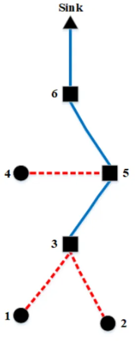
In W the number of nodes and positions are fixed. In order to achieve the goal of this work W is partitioned into two sets of nodes, cluster heads (CH) and member nodes (B). Using these sets of nodes two subgraphs of W are defined; BLUE and RED as shown below.
𝐵𝐵𝐵𝐵𝐵𝐵𝐸𝐸 = (𝐶𝐶𝐻𝐻 ∪ 𝑆𝑆,𝐸𝐸𝐵𝐵𝐵𝐵𝐵𝐵𝐵𝐵) 𝑤𝑤ℎ𝑒𝑒𝑒𝑒𝑒𝑒𝐸𝐸𝐵𝐵𝐵𝐵𝐵𝐵𝐵𝐵 ⊂ 𝐸𝐸
𝑅𝑅𝐸𝐸𝑅𝑅 = (𝐵𝐵 ∪ 𝐶𝐶𝐻𝐻,𝐸𝐸𝑅𝑅𝐵𝐵𝑅𝑅) 𝑤𝑤ℎ𝑒𝑒𝑒𝑒𝑒𝑒𝐸𝐸𝑅𝑅𝐵𝐵𝑅𝑅 ⊂ 𝐸𝐸𝑎𝑎𝑚𝑚𝑑𝑑 ∀ (𝑣𝑣,𝑤𝑤)∈ 𝐸𝐸𝑅𝑅𝐵𝐵𝑅𝑅:𝑣𝑣 ∈ 𝐵𝐵𝑎𝑎𝑚𝑚𝑑𝑑𝑤𝑤 ∈ 𝐶𝐶𝐻𝐻
CH nodes receive messages from B nodes that are connected to them via the RED graph. Messages are transmitted from CH nodes to the sink(s) via the BLUE graph.
In order to be considered feasible the network graph W has to provide for the communication of all nodes to a sink. In order for this to be true both the BLUE and RED
partitions have to be feasible. The BLUE graph is feasible if and only if all CHs are connected through the BLUE graph to a sink node. The RED graph is feasible if and only if all member nodes(B) are connected to a cluster head(CH).
Using the above definitions there are potentially many feasible partitions of W into RED
and BLUE. Different partitions result in different energy consumption rates and therefore a longer or shorter network lifetime. The target function TF(), detailed in the formal definition below, is used to calculate the energy consumed by the network over a fixed period of time. The optimal partition of W into RED and BLUE minimizes the target function and thereby results in the longest network lifetime. A formal definition of the problem follows below.
Formal Definition
Given a set of nodes V = {𝑣𝑣𝑖𝑖 | 1≤ 𝑚𝑚 ≤ 𝑚𝑚} in an undirected graph G and an integer m, such that 0<m<n, the problem is to partition V into m clusters (C1, C2, …, Cm) and to identify cluster heads𝐶𝐶𝐻𝐻= {𝑐𝑐ℎ𝑖𝑖|1≤ 𝑚𝑚 ≤ 𝑚𝑚,𝑐𝑐ℎ𝑖𝑖 ∈ 𝑉𝑉}. The resulting network configuration shall be such that each cluster has exactly one cluster head, there exists a path from all nodes to a sink,
15
and the target function TF() is minimized. The set of sink nodes S is defined as 𝑆𝑆= {𝑠𝑠𝑖𝑖|1≤ 𝑚𝑚 ≤ 𝑐𝑐,𝑠𝑠𝑖𝑖 ∉ 𝑉𝑉} where c indicates the number of sinks.
Distance within the wireless sensor network is defined as three-dimensional Euclidean distance. The distance between two nodes 𝑞𝑞 ∈ 𝑉𝑉and p∈ 𝑉𝑉 is therefore given by:
𝑑𝑑(𝑞𝑞,𝑝𝑝) =�(𝑞𝑞𝑥𝑥− 𝑝𝑝𝑥𝑥)2+ (𝑞𝑞𝑦𝑦− 𝑝𝑝𝑦𝑦)2+ (𝑞𝑞𝑧𝑧−𝑝𝑝𝑧𝑧)2 (2)
Using the distance function, MAconnect, the function that identifies if nodes are connected by an edge is defined below.
𝑀𝑀𝑀𝑀𝑐𝑐𝑜𝑜𝑜𝑜𝑜𝑜𝑐𝑐𝑐𝑐𝑐𝑐(𝑣𝑣𝑖𝑖,𝑣𝑣𝑗𝑗) =�0 ; 1 ; 𝑑𝑑𝑑𝑑((𝑣𝑣𝑣𝑣𝑖𝑖,𝑣𝑣𝑗𝑗) ≤ 𝑅𝑅
𝑖𝑖,𝑣𝑣𝑗𝑗) >𝑅𝑅 (1)
The graph partition can be converted into partition of two subgraphs, BLUE and RED. The
BLUE graph represents the cluster heads (CHs), connections between CHs, and connections from
CHsto sinks. The REDgraph represents the member nodes 𝐵𝐵= {𝑏𝑏𝑖𝑖|1≤ 𝑚𝑚 ≤ 𝑚𝑚,𝑏𝑏𝑖𝑖 ∈ 𝑉𝑉,𝑏𝑏𝑖𝑖 ∉
𝐶𝐶𝐻𝐻} and connections from member nodes to CHs. The REDgraph is feasible if and only if all of the nodes in the REDgraph are connected to a CH. Using MAconnect above, a Boolean function RED() can be defined as:
𝑅𝑅𝐸𝐸𝑅𝑅(𝐵𝐵) =�𝑡𝑡𝑒𝑒𝑡𝑡𝑒𝑒 ; 𝑚𝑚𝑖𝑖∀𝑏𝑏 ∈ 𝐵𝐵:∑𝑚𝑚𝑖𝑖=1𝑀𝑀𝑀𝑀𝑐𝑐𝑜𝑜𝑜𝑜𝑜𝑜𝑐𝑐𝑐𝑐𝑐𝑐(𝐶𝐶𝐻𝐻𝑖𝑖,𝑏𝑏) ≥ 1
𝑖𝑖𝑎𝑎𝑓𝑓𝑠𝑠𝑒𝑒 ; 𝑜𝑜𝑡𝑡ℎ𝑒𝑒𝑒𝑒𝑤𝑤𝑚𝑚𝑠𝑠𝑒𝑒 (3) The above equation indicates that the REDgraph is feasible if and only if all member nodes are within transmission range of at least one cluster head. The BLUE graph is feasible if and only if all CHsare connected through the BLUE graph to a sink node 𝑠𝑠 ∈ 𝑆𝑆as indicated in equation (4) below. In equation (4), Scomp represents the set of nodes that form the component of the sink(s).
16
𝐵𝐵𝐵𝐵𝐵𝐵𝐸𝐸(𝐶𝐶𝐻𝐻) =�𝑖𝑖𝑎𝑎𝑓𝑓𝑠𝑠𝑒𝑒𝑡𝑡𝑒𝑒𝑡𝑡𝑒𝑒 ; ; 𝑚𝑚𝑖𝑖𝑜𝑜𝑡𝑡ℎ𝑒𝑒𝑒𝑒𝑤𝑤𝑚𝑚𝑠𝑠𝑒𝑒∀𝑐𝑐ℎ ∈ 𝐶𝐶𝐻𝐻 : 𝑐𝑐ℎ ∈ 𝑆𝑆𝑐𝑐𝑜𝑜𝑚𝑚𝑝𝑝 (4) Initially in this work network configurations will only be considered feasible if all sinks are connected to the same component. Sinks with separate components are considered separate networks. It is feasible that there exist network topologies such that separate sink components facilitate less overall energy usage and additional work to explore this may be done in the future.
The function that defined the energy consumption of a wireless sensor network over a given time interval is expressed as 𝑖𝑖(𝐸𝐸𝑟𝑟𝑐𝑐𝑐𝑐𝑣𝑣,𝐶𝐶𝐻𝐻), where Erecv is the energy consumed by a node to receive a message. The function is defined below for a finite time period that is a small fraction (<1%) of the typical network lifetime.
𝑖𝑖(𝐸𝐸𝑟𝑟𝑐𝑐𝑐𝑐𝑣𝑣,𝐶𝐶𝐻𝐻) =�[
𝑥𝑥
𝑚𝑚∗
𝐸𝐸𝑠𝑠𝑐𝑐𝑜𝑜𝑠𝑠+𝑦𝑦𝑖𝑖 ∗ 𝐸𝐸𝑟𝑟𝑐𝑐𝑐𝑐𝑣𝑣] +𝑒𝑒|𝐶𝐶𝐻𝐻| 𝑚𝑚𝑚𝑚=1
=∑𝑚𝑚𝑚𝑚=1[
𝑥𝑥
𝑚𝑚∗ 𝑘𝑘
+𝑦𝑦𝑖𝑖]∗ 𝐸𝐸𝑟𝑟𝑐𝑐𝑐𝑐𝑣𝑣+𝑒𝑒|𝐶𝐶𝐻𝐻| (5)In equation (5) the variables 𝑥𝑥𝑖𝑖 and 𝑦𝑦𝑖𝑖 represent the number of messages being sent and received at 𝑣𝑣𝑖𝑖 respectively. The constant k is a factor representing the extra energy required to send versus receive transmissions as defined in (Wu et al., 2002).
𝐸𝐸𝑠𝑠𝑐𝑐𝑜𝑜𝑠𝑠 =𝑘𝑘𝐸𝐸𝑟𝑟𝑐𝑐𝑐𝑐𝑣𝑣, 𝑘𝑘 ≥1(Wu et al., 2002)
The last variable e accounts for the extra energy consumed by cluster heads versus member nodes. It represents the energy required for the average cluster head to maintain routing information and actively listen for messages from member nodes. Sinks are typically connected
17
to a substantial power source and are therefore not considered in the problem to minimize the energy usage of the network.
Given the above, the target function TF() to be minimized in this work can now be defined for a given network configuration as shown in equation (6) below.
𝑇𝑇𝑇𝑇() = � 𝑖𝑖∞( ; 𝐸𝐸𝑟𝑟𝑐𝑐𝑐𝑐𝑣𝑣,𝐶𝐶𝐻𝐻) ; 𝑜𝑜𝑡𝑡ℎ𝑒𝑒𝑒𝑒𝑤𝑤𝑚𝑚𝑠𝑠𝑒𝑒𝑚𝑚𝑖𝑖𝑅𝑅𝐸𝐸𝑅𝑅(𝐵𝐵) = 𝑡𝑡𝑒𝑒𝑡𝑡𝑒𝑒𝑀𝑀𝐴𝐴𝑅𝑅𝐵𝐵𝐵𝐵𝐵𝐵𝐸𝐸(𝐶𝐶𝐻𝐻) =𝑡𝑡𝑒𝑒𝑡𝑡𝑒𝑒 (6) As defined in equation (6), the energy definition function 𝑖𝑖(𝐸𝐸𝑟𝑟𝑐𝑐𝑐𝑐𝑣𝑣,𝐶𝐶𝐻𝐻), is only valid when the network is feasible, meaning that all nodes are able to communicate through a path with at least one sink. A network configuration is considered feasible when the RED graph is feasible, and the BLUE graph is feasible. When a network configuration is not feasible, meaning either the
REDor BLUE graph are not feasible, then the configuration receives infinity as the score. Since this is a minimization problem, infinity indicates the poorest performance for a configuration.
The problem as presented above shows that the p-median problem can be constrained in a manner to emulate a WSN and therefore the work presented here on improving the lifetime of a WSN may be extended to be applicable to a greater class of problems.
Dissertation Goal
As the literature review below shows, many clustering algorithms for WSNs were successful in reducing network overhead or improving resource utilization as compared to the existing protocols. However, the success occurs typically only within a certain range of
environmental factors such as a mostly static network (Wu, Cao & Raynal, 2009), greater than a certain number of nodes (Chauhan, Awasthi, Chand & Chugh, 2011), or within a certain
18
It is also shown in the literature review that there are several common characteristics that are desirable for a WSN clustering algorithm:
• It should improve network scalability by reducing network overhead associated with routing messages (Er & Seah, 2010).
• It should reduce energy consumption via lower computational overhead, thereby improving the lifespan of nodes with limited battery power (Chauhan et al., 2011).
• It should improve the successful delivery of packets (Safa et al., 2010).
• It should not significantly increase overall network resource usage due to cluster maintenance (Zhang et al., 2009).
The goal of this research was to develop a clustering method to prolong the lifetime of a WSN. This meant reducing the overall resource usage of the network without negatively impacting the delivery of packets. These characteristics were satisfied over a wide range of environments. The measurement of success was through reducing power usage and prolonging the network lifetime. Improving scalability and packet delivery are beyond the scope of this work.
Research Questions
As can be seen in the literature there have been many attempts to improve clustering of WSNs. The research questions that arise from a review of the literature involve attempts to provide meaningful comparisons to this existing body of work and also improvements upon it. Therefore, the primary questions to be addressed by this research are as follows:
19
2. Is it possible to adapt a genetic algorithm to identify clusters in WSNs? 3. Is there value in considering a WSN a capacitated p-median problem?
4. Can a genetic algorithm optimize clustering of a WSN when the nodes have variable transmission range?
Relevance and Significance
As noted earlier there are many practical applications for WSNs including military and emergency or rescue situations (Abbasi & Younis, 2007). In both these situations maintaining communications is critical. Soldiers need to maintain communication to coordinate their
movements and alert others to danger. Reducing the resource usage of WSN nodes would allow soldiers to stay in communication longer. Cluster head schemes would also provide the node management and communication required for improved intrusion detection (Zhang & Lee, 2000). Similarly, in rescue operations, allowing rescue workers to stay in communication longer would facilitate longer search and rescue operations. The proposed research benefits both these implementations as well as other situations where a low-cost network that can be set up quickly is required.
Much of the previous work related to clustering algorithms for WSNs has focused on particular performance aspects. Some focused on reducing routing overhead through a reduction in the number of routing messages. Other work focused on power usage, attempting to keep nodes active as long as possible by reducing CPU load to preserve battery life. There are also examples where cluster overhead was the focus as compared to other clustering algorithms or protocols. When compared to more commonly used protocols and clustering schemes in
previous work, many of these more recent approaches were successful in improving a particular aspect of WSN performance. While all of these aspects are important, trade-offs were often
20
necessary to achieve a singular goal. This dissertation focused on power usage of WSNs in order to prolong the lifetime of the network. However, rather than focusing on one aspect of power usage, this work evaluated the most important factors in power consumption. Factors considered in power consumption included message delivery efficiency and cluster management overhead.
Additionally, the overall power usage of the network was considered using different clustering schemes. This comparison was required since different schemes resulted in different numbers of nodes being in an active versus passive mode and also changed the amount of network maintenance required at each individual node. The relative power usage of each factor was compared and the work focused on the factors determined to be significant in prolonging the life of the network through reduced power consumption. The significant result of this research was an algorithm that improved network energy wfficiancy across a range of environments.
It is likely that much of this work may be applicable in other situations. Any
circumstance where clustering of data points is required could benefit from this work. This work will also be useful in the broader field of location problems such as the p-median problem.
Barriers and Issues
There are several factors that make developing an ideal clustering system for wireless sensor networks (WSNs) inherently difficult. As noted above, finding the optimal clustering solution is in general an NP-hard problem. Therefore, the clustering solution was difficult to measure since brute force methods even on a small p-median problem are not feasible. There are p-median problem data sets with known optimal solutions but these are not constrained as would make them applicable for WSNs. Also, any solution must be scalable, since WSNs may scale up to thousands of nodes depending on the application (Abbasi & Younis, 2007).
21
Along with the primary task of developing the clustering algorithm there are peripheral issues that complicated the proposed work. There is no standard set of benchmarks to test the implementations against. Therefore, a reasonable set of metrics had to be developed as part of the work.
Assumptions, Limitations and Delimitations
Assumptions. Within the context of this work it was assumed that the sensor nodes being modeled were in good working order and functioning per design. There existed no defects in the nodes that caused them to lose power prematurely or have their power drained due to reasons other than operations used in typical network operations such as sending and receiving messages and maintaining routing information as applicable. The nodes were also expected to be of the same type and manufacture so that they all had the same transmission range and consumed the same amount of power for the same operations. It was also assumed that wireless transmissions sent by nodes were received by nodes within range and were not blocked or corrupted due to environmental or other external conditions. While variable transmission distances and power levels may be modeled in future work, this assumption eliminated the need to account for resending a proportion of messages. Also it was assumed that the sink had sufficient computing power to perform the clustering calculations in a reasonable time.
The assumptions of no defects in the nodes and 100% successful message transmission may not be typical of what is encountered in real-world situations. However, these assumptions did not affect the results of the work being proposed. The intention was that these assumptions were held true for all network clustering schemes being compared and therefore they did not provide an advantage to one scheme over another. The assumption that all nodes were the same was not unreasonable given that the nodes of a network will typically be deployed to monitor the
22
same values; temperature, seismic, motion, etc., and therefore using the same type and
manufacture of node would reduce variability among the data collected from different nodes. The last assumption related to computing power at the sink was not unreasonable since a standard PC should provide sufficient power for the calculations required.
Limitations. The primary limitation for this work was the lack of relevant solved data sets. Although there are solved data sets for the p-median problem where the optimal
configuration is provided, they do not include the constraints given in the problem statement for this proposed work in order to make the solution applicable for WSNs. The intent of this work was to ultimately compare the results of various clustering schemes and therefore this limitation did not affect the validity of the work. However it should be known how close the proposed solution is to providing theoretical optimal solutions.
An additional limitation of the proposed work was that the feasibility of the solution will only be tested using software simulations of WSNs. A real-world test of the proposed solution was not feasible due to time and resource constraints. This did not reduce the validity of the work since this is typically the case for similar approaches in the literature and the comparisons of different approaches were performed using similar methodologies.
Delimitations. In order to make the p-median problem applicable to WSNs the networks were constrained to have cluster sizes no larger than a fixed-radius, meaning that the radius of any cluster could not be larger than the transmission range of the nodes. In order to facilitate communication between clusters the distance between cluster heads was also constrained to less than twice the transmission range. Also each cluster had to have exactly one cluster head and
23
each node had to belong to at least one cluster. Additionally this research only considered networks with one sink.
Summary
Wireless sensor networks (WSNs) have been shown to be useful in many situations where a network needs to be set up quickly and no fixed infrastructure exists. The individual sensor nodes of a WSN are typical small devices that rely upon battery power. Therefore there has been much work done toward the goal of reducing the power usage of the individual nodes and thereby prolonging the lifetime of the network. One method of reducing power usage of a WSN is to cluster the nodes and assign a cluster head for each cluster. A cluster head maintains routing information and combines messages from the nodes within its cluster. It has been shown that machine learning techniques are applicable to determining the optimal cluster configuration. The method that was focused on in this work was a genetic algorithm.
The problem of clustering the nodes of a WSN can be considered a constrained version of a larger class of problems known as location problems and more specifically the p-median
problem. The p-median problem is the problem of locating facilities so that there is minimal cost of travel for all demand units. The cluster heads within a WSN can be considered the facilities with the remaining nodes of the WSN the demand points. In order to approach the node
clustering problem as an optimization problem like the p-median problem, a target function was created that included terms for network architecture and location of cluster heads as well as the energy required for sending and receiving message and the number of messages sent.
Constraints on the problem included limiting the radius of clusters to the transmission range of the nodes, requiring that each cluster has exactly one cluster head, and that each node belong to at least one cluster.
24
There are several difficulties in clustering the nodes of a WSN. Finding the optimal cluster configuration of a network is an NP-hard problem and a brute force approach will not work even with a small network. Also, there does not exist a set of solved problems to benchmark results against therefore the proposed solution had to be compared to other approaches.
25
Review of the Literature
The literature review is presented in three sections. The first section covers the p-median problem. The next section presents wireless sensor networks and mobile ad hoc networks. The final section covers potential machine learning approaches.
P-median
The p-median section of the literature review begins with papers that provide the
foundation of the p-median problem. The subsequent papers reviewed demonstrate that machine learning techniques such as genetic algorithm and neural network are viable methods for
obtaining p-median optimizations.
Hakimi (1964) is an early study on the problem of finding the center and median of a graph G where the edges and vertices are weighted. The problem is modeled as finding the ideal location of a switching center S in a communications network. The optimal location was where the length of connections from all vertices to S was minimized and this location was called the
absolute median of the graph. Finding the absolute center of a graph is also discussed but is less relevant to this work and therefore not detailed here.
The work by Hakimi (1964) begins with definitions. The graph G is said to contain vertices v and branches b with weights hi and wi associated with vertices and branches
respectively. The length of a path between two points on G is defined as the sum of the weights of the branches along the path and the distance between any two points 𝑑𝑑(𝑥𝑥,𝑦𝑦) was defined as the minimum length path between the points. Given these definitions the absolute median was defined as a point y0 “if for every point y on G” (Hakimi, 1964):
26
The work in Hakimi (1964) continues with providing a proof for the theorem that the absolute median of a graph must be at one of the vertices. The proof begins by substituting in the definition above and stating that for an arbitrary point x0 on G where x0 is not a vertex, there “exists a vertex vm such that” (Hakimi, 1964):
∑𝑜𝑜𝑖𝑖=1ℎ𝑖𝑖𝑑𝑑(𝑣𝑣𝑖𝑖,𝑥𝑥0)≥∑𝑖𝑖=1𝑜𝑜 ℎ𝑖𝑖𝑑𝑑(𝑣𝑣𝑖𝑖,𝑣𝑣𝑚𝑚) (Hakimi, 1964) (8)
The point x0 is said to be on a branch 𝑏𝑏(𝑣𝑣𝑝𝑝,𝑣𝑣𝑞𝑞)of G. The distance of any vertex vi
will be the minimum of the distance to either vp or vq plus the distance to x0:
𝑑𝑑(𝑣𝑣𝑖𝑖,𝑥𝑥0) = min [𝑑𝑑�𝑥𝑥0,𝑣𝑣𝑝𝑝�+𝑑𝑑�𝑣𝑣𝑝𝑝,𝑣𝑣𝑖𝑖�,𝑑𝑑�𝑥𝑥0,𝑣𝑣𝑞𝑞�+𝑑𝑑(𝑣𝑣𝑞𝑞,𝑣𝑣𝑖𝑖)] (Hakimi, 1964) (9)
Equation (8) is substituted into equation (9) so that two equations result. It is then shown through additional substitution that both cases show that equation (7) is true. Therefore, it was proven that the absolute median was a vertex on the graph G (Hakimi, 1964).
The work in Hakimi (1964) is important in providing a foundation for future work on the p-median problem. It allowed for limiting the points considered as the median of a graph to the vertices. This work was extended to show that the solution to the p-median problem would consist of points on the vertices of a graph in Hakimi (1965) reviewed next.
Hakimi (1965) begins considering the same problem as above except in this case the problem was expanded from finding the ideal location for a single switching center S to multiple switching centers S1, S2, …, Sp. The network was again considered a graph G with weights attached to the branches and vertices. Distance between points was defined the same as above. Given a set of points , x1, x2, …, xp, that represent the switching centers on G, Xp* is considered a p-median if for all possible Xp:
27
∑𝑜𝑜𝑖𝑖=1ℎ𝑖𝑖𝑑𝑑(𝑣𝑣𝑖𝑖,𝑋𝑋𝑝𝑝∗)≤∑𝑜𝑜𝑖𝑖=1ℎ𝑖𝑖𝑑𝑑(𝑣𝑣𝑖𝑖,𝑋𝑋𝑝𝑝) (Hakimi, 1965)
The distance 𝑑𝑑(𝑣𝑣𝑖𝑖,𝑋𝑋𝑝𝑝) was defined as the distance from vi to the nearest member of Xp. This work also considered the problem of finding the p-centers that is less relevant to this work and not reviewed in detail.
Hakimi (1965) next walked through a proof building on the one in Hakimi (1964) that showed that within the set of vertices V on G “there exists a subset Vp* of V containing p vertices such that for every set of p points X on G” (Hakimi, 1965):
∑𝑜𝑜𝑖𝑖=1ℎ𝑖𝑖𝑑𝑑(𝑣𝑣𝑖𝑖,𝑋𝑋) ≤∑𝑜𝑜𝑖𝑖=1ℎ𝑖𝑖𝑑𝑑(𝑣𝑣𝑖𝑖,𝑉𝑉𝑝𝑝∗) (Hakimi, 1965)
Similar to the finding above, this proof showed that the set of points that make up the p-median are a subset of the set of vertices V of the graph. Therefore, when considering the solution for a location problem such as the ideal location for switching centers only graph vertices need to be considered (Hakimi, 1965).
Hakimi (1965) also presented a numerical method for finding the p-median. The sample problem was finding the optimal location of three switching centers within a network that contained n nodes. The solution included first creating an n x n distance matrix of the nodes on
G. The distance matrix was then multiplied by the weight of the corresponding vertex. Next the sum:
∑ min (𝑑𝑑𝑖𝑖𝑟𝑟∗ ,𝑑𝑑
𝑗𝑗𝑟𝑟∗,𝑑𝑑𝑘𝑘𝑟𝑟∗ ) 𝑜𝑜
𝑟𝑟=1
was calculated for all possible values of i, j, and k where (1≤ 𝑚𝑚,𝑗𝑗,𝑘𝑘 ≤ 𝑚𝑚). The values where the above sum was a minimum were those that were selected for the switching centers (Hakimi, 1965).
28
Hakimi (1965) extended the work of Hakimi (1964) and proved that a p-median of a graph exists such that the points that make up the p-median are vertices of the graph. A numerical method was presented for finding the p-median of a small directed graph which showed the complexity of the problem. This work provided the foundation for subsequent heuristic-based approaches to finding the p-median of a graph.
Correa, Steiner, Freitas & Carnieri (2004) proposed using a genetic algorithm for solving a constrained version of the p-median problem. In their work the constraints involved solving a capacitated version of the p-median problem. P-median problems are generally presented as finding the optimal locations for a fixed number of facilities to minimize the distance to demand nodes on a graph. In typical p-median problems the facilities can supply an unlimited number of demand nodes, however in the capacitated version the supply from each facility is limited. An additional constraint that is similar to this work was that each demand node had to be associated with exactly one facility (Correa et al., 2004).
Correa et al. (2004) applied their work to a real-world scenario. Their problem consisted of 43 potential testing facilities that needed to supply the demand from 19,710 students. The goal was to choose the facilities that would minimize the distance from students’ homes to their respective testing facility. It was predetermined that a subset of 26 facilities would be used to supply the demand. Correa et al. (2004) implemented a genetic algorithm to optimize the solution.
A typical genetic algorithm (GA) is a machine learning optimization algorithm that begins with random solutions, each one known as a chromosome. The GA then selects the best candidate chromosomes based on a fitness function and uses those to create the next generation
29
of chromosomes (Whitley, 1994). The chromosomes are combined using a probability-based crossover function that selects random members (genes) from two parent chromosomes and swaps them. Chromosomes are also altered through a mutation method that randomly changes genes within the chromosome. Mutation is also based on probability and the mutation
probability is typically much lower than the crossover probability (Whitley, 1994). This process successively creates generations that are a better solution that the previous genera ration. This process generally continues for a predetermined number of generations or a specific fitness threshold is reached (Whitley, 1994).
The GA used in Correa et al. (2004) was modified to better fit the problem space. Each chromosome was a set of 26 indices that represented the ID of a particular facility. The fitness of each chromosome was measured by the total sum distance of all students from their assigned facility. The assignment process began by assigning each student to the nearest facility as long as that facility had capacity. Afterward the student was assigned to the next nearest facility with capacity until all students were assigned. After assignment was complete students not assigned to the nearest facility were exchanged and the total sum distance recalculated to determine if the exchange improved the solution. Improvements were retained and this process continued until the solution was no longer improved (Correa et al., 2004).
The crossover method implemented by Correa et al. (2004) removed duplicate facility indices so that no solution could have the same facility included more than once. A random number was used to determine the number of genes that were swapped. A heuristic was applied to the mutation method based on domain knowledge. A percentage of chromosomes were randomly selected and then each gene of the chromosome was replaced with a facility index not currently in the chromosome. If the change improved the fitness of the chromosome, then it was
30
retained. Finally, no chromosomes were added to the next generation if their fitness was no better than the worst performing chromosome of the previous generation (Correa et al., 2004).
Correa et al. (2004) tested their algorithm with and without the mutation heuristic and tested against the tabu search algorithm. In the tabu search algorithm a set of facilities were first randomly selected. Then the solution was iterated by either adding, dropping, or swapping facilities. Each operation was evaluated so that the facility that provided the minimum sum distance was used in the operation. This process was repeated for a predetermined number of iterations (Correa et al., 2004). The number of iterations for the two versions of the GA was adjusted to make the computational time roughly equivalent between both Gas and the tabu search. The version with heuristic mutation used 1,000 iterations. The heuristic mutation was very computationally expensive and the GA without it used 12,100 iterations with the runtime of the two GAs found to be similar. The tabu search used 150 iterations which resulted in a run time similar to the two GAs. The three algorithms had similar results based the total sum distance and the percentage of students assigned to the nearest facility. The GA with heuristic mutation performed the best with total distance of 45,999 km and 83% of students assigned to the nearest facility. The tabu search was next with 46,660 km total distance and 82% of students assigned to the nearest facility. The GA without heuristic mutation had a total distance of 47,313 km and 79% of students assigned to the nearest facility. The results showed that all three
performed well and that the heuristic mutation is a viable method for improving the GA performance (Correa et al., 2004).
The work by Correa et al. (2004) showed that the GA can provide a good solution for the p-median problem. The constraint of having each student assigned to exactly one facility is
31
similar to this work and therefore may provide insight into a possible solution. There may be a heuristic mutation for the wireless sensor network problem space that improves the solution.
Domínguez & Muñoz (2008) proposed using a recurrent neural network to solve a constrained version of the median problem. Their work begins with reiterating that the p-median problem is NP hard and the authors list several heuristic methods from the literature. Next a brief description of neural networks (NN) is provided. It begins by stating that NNs are a viable solution for many different types of problem including pattern classification, clustering and combinatorial optimization. A binary artificial neuron was described as having an activation value that results in output of either 1 or 0. A recurrent neural network is described as a set of N
artificial neurons connected by links that each have a weight associated with them. The concept of an energy function is introduced and provided as:
𝐸𝐸(𝑡𝑡) =−12∑𝑁𝑁𝑖𝑖=1∑𝑁𝑁𝑗𝑗=1𝑤𝑤𝑖𝑖𝑗𝑗𝑥𝑥𝑖𝑖(𝑡𝑡)𝑥𝑥𝑗𝑗(𝑡𝑡)+∑𝑁𝑁𝑖𝑖=1𝜃𝜃𝑖𝑖𝑥𝑥𝑖𝑖(𝑡𝑡) (Domínguez & Muñoz, 2008)
In the equation above, 𝑤𝑤𝑖𝑖𝑗𝑗 represents the weight of the connection between neurons i and j. The term “𝑥𝑥𝑖𝑖(𝑡𝑡) is the activation value of neuron i at time t, and 𝜃𝜃𝑖𝑖 is the threshold value for the neuron I” (Domínguez & Muñoz, 2008). The energy function will either stay the same or
decrease and when the energy function is stable it indicates the network has reached a minimum. It was also noted that these types of recurrent neural networks, also known as Hopfield networks, tend to settle into a local minimum versus a global minimum (Domínguez & Muñoz, 2008).
Domínguez & Muñoz (2008) next define the constraints applied to the p-median problem. Given a system with n demand nodes and p facilities the problem was to minimize:
32
In the equation above, dij is the distance between the demand point i and the facility j. The terms
xiq and yjq represented allocation variables and location variables respectively. The allocation and location variables were defined by:
𝑥𝑥𝑖𝑖𝑞𝑞 =�1 if 0 otherwise,𝑚𝑚 is assigned to cluster 𝑞𝑞, (Domínguez & Muñoz, 2008) 𝑦𝑦𝑗𝑗𝑞𝑞 = �1 if 0 otherwise,𝑗𝑗 is the center of cluster 𝑞𝑞, (Domínguez & Muñoz, 2008)
The first constraint was that each demand node was a member of only one cluster and was expressed as:
∑𝑝𝑝𝑞𝑞=1𝑥𝑥𝑖𝑖𝑞𝑞 = 1, 𝑚𝑚= 1, … ,𝑚𝑚, (Domínguez & Muñoz, 2008)
The second constraint was that each cluster must contain exactly one facility and was expressed as:
∑𝑜𝑜𝑗𝑗=1𝑦𝑦𝑗𝑗𝑞𝑞 = 1, 𝑞𝑞= 1, … ,𝑝𝑝, (Domínguez & Muñoz, 2008)
The constraints were included as a penalty value in the energy equation in order to express the problem as unconstrained. This yielded the energy equation below:
𝐸𝐸 =∑𝑖𝑖=1𝑜𝑜 ∑𝑗𝑗=1𝑜𝑜 ∑𝑝𝑝𝑞𝑞=1𝑑𝑑𝑖𝑖𝑗𝑗𝑥𝑥𝑖𝑖𝑞𝑞𝑦𝑦𝑗𝑗𝑞𝑞+𝜆𝜆1∑ �𝑜𝑜𝑖𝑖=1 1− ∑𝑝𝑝𝑞𝑞=1𝑥𝑥𝑖𝑖𝑞𝑞�2 +𝜆𝜆2∑𝑝𝑝𝑞𝑞=1�1− ∑𝑜𝑜𝑗𝑗=1𝑦𝑦𝑗𝑗𝑞𝑞�2
33
The 𝜆𝜆𝑖𝑖 > 0 parameters represent the weight of the penalty term and it is noted that finding proper values for the penalty weights is an “important problem associated with this approach”
(Domínguez & Muñoz, 2008).
In order to avoid the problem of tuning the penalty parameters, Domínguez & Muñoz (2008) structured their neural network in such a manner so that the architecture of the network enforced the constraints. This was accomplished through constructing the network as a set of disjoint groups where for n demand points there were n groups with only one neuron in each group allowed to be active at any time. Similarly, for p facility locations there were p groups also with only one neuron allowed to be active. In this manner, the constraints were satisfied through the network architecture and the penalty terms could be removed from the energy equation which resulted in the simplified equation:
𝐸𝐸= ∑𝑜𝑜𝑖𝑖=1∑𝑜𝑜𝑗𝑗=1∑𝑝𝑝𝑞𝑞=1𝑑𝑑𝑖𝑖𝑗𝑗𝑥𝑥𝑖𝑖𝑞𝑞𝑦𝑦𝑗𝑗𝑞𝑞 (Domínguez & Muñoz, 2008)
34
Figure 4. Disjoint Groups (Domínguez & Muñoz, 2008)
Domínguez & Muñoz (2008) implemented two different algorithms for updating the network. Group-parallel dynamics (NA-G) updated one group at a time while layer-parallel dynamics (NA-L) updated all groups in a layer at the same time. The two algorithms were tested on a set of p-median problems with known optimal solutions. It was found that the results from both were relatively poor and this was discovered to be due to the initial selection of the facility locations. An additional scattering algorithm was added to NA-L to set the initial locations of the facilities and this improved the performance of the algorithm but also significantly increased computational overhead. The new algorithm, NA-L+ , was tested against the known heuristic method variable neighborhood search (VNS). The computational time of VNS was limited to be similar to the time of NA-L+. With this constraint, NA-L+ obtained superior optimization on almost all of the test scenarios. This showed that the neural network approach was a viable
35
method for finding the p-median and that it was able to do so in less time computationally (Domínguez & Muñoz, 2008).
This work presented in (Domínguez & Muñoz, 2008) is important for this work since the constraints are identical and the authors were able to implement a machine learning method to find optimal p-median solutions. IT is unknown if the VNS algorithm would ultimately have found better solutions given more run time and will be interesting to compare the solution proposed in this work to VNS in terms of solution quality and run time.
Wireless sensor networks and MANETs
As noted above wireless sensor networks (WSNs) represent a special case of mobile ad hoc networks (MANETs). There are two primary differences between WSNs and MANETs. The first is that in MANETs the nodes are typically mobile whereas in WSNs they are not. There may be some node mobility in WSNs such as sensors floating in the ocean on currents, but generally this movement is not significant as compared to the mobility of MANET nodes. The other difference is the existence of the base-station or sink in a WSN. MANET nodes typically only communicate with each other but WSNs send information to a sink that then transmits the information to other systems where it is consumed. Otherwise the two networks present many of the same problems including limited battery power of devices and the requirement for the
network to be set up quickly without pre-existing infrastructure. Therefore, most of the solutions presented for MANETs are also applicable to WSNs.
Drugan et al. (2011) proposed implementing a clustering method based on work done in identifying communities such as social networks. The reasoning behind this approach was that clusters could be identified based on routing information and therefore no additional
36
communication overhead would be added for cluster discovery and maintenance. It is
acknowledged by the authors that sparse MANETs pose additional problems versus systems with large numbers of data points and therefore the methods used for larger numbers of objects must be modified for use with sparse MANETs (Drugan et al., 2011).
The approach is based on the underlying assumption that areas of nodes with dense connections to each other represent communities or clusters and that individual clusters will have fewer connections between them (Drugan et al., 2011). This is relevant to the work proposed in this dissertation since this approach, although relying on network connections instead of node location is a method to measure of node density. Drugan et al. (2011) also use k-medoids as an algorithm for comparison and point out the shortcoming of k-medoids that it requires a
predetermined number of clusters in order to operate. The authors implement several different community detection algorithms make minor adjustments to the algorithms to account for detection of clusters in sparse data. The algorithms implemented included a modularity- based algorithm: Newman and Griven Community Detection, random walk algorithm: vanDongen Community Detection, and potts-based: Reichard and Bornholdt Community Detection (Drugan et al., 2011).
Drugan et al. (2011) explain the different types of routing protocols typically used in MANETs. There are reactive protocols that perform route discovery when communication is required and proactive protocols that maintain routing information and update it periodically. Optimized Link State Routing (OLSR) is a proactive protocol. OLSR is ideal for “large and dense mobile networks” (Clausen & Jacquet, 2003). Individual nodes maintain routing tables of network topology that is shared by other nodes. Using this information each node can use the information it has stored locally to route packets. OLSR also makes use of nodes that are
37
designated as multipoint relays (MPRs). A node designates its one-hop neighbors that it can establish two-way communication with as MPRs. MPRs broadcast to the network that they can reach the nodes that have designated them as MPRs and also are responsible for network control traffic. In this manner OLSR is able to reduce the amount of flooding traffic required to
maintain network routing paths (Clausen & Jacquet, 2003).
The algorithms were all evaluated using Global Mobile Information System Simulation Library network simulation. The OLSR protocol was used along with both static and mobile network nodes. It was also assumed that 25% of the nodes would send communications every 5 seconds. Forty nodes were used in the simulation in an area of 800m x 600m and the mobility of the dynamic nodes varied from 1m/s to 7m/s and a node transmission range of 100 m (Drugan et al., 2011).
The Silhouette index was used to measure the quality of clustering. It was developed by Rousseeuw (1987) as part of a method to graphically determine the quality of clusters and also help determine if the appropriate number of clusters was created from a set of points. The creation of a silhouette depended on the calculation of an index value denoted s(i). Other values calculated were the dissimilarity of a node to its associated cluster, a(i), and dissimilarity with the next nearest cluster, b(i) . In Figure 5 below a(i) is the average distance of the point i to the other points in the cluster of which it is a member, in this case cluster A. The value b(i) is the average distance to points in the next nearest cluster, in this case cluster B (Rousseeuw, 1987).
38
Figure 5. Clusters (Rousseeuw, 1987)
The value for s(i) can then be calculated using Equation (10) below. Per Equation (10), s(i) will vary from values of -1 to 1, with 1 indicating that the node i is well clustered while a value of s(i)
closer to -1 indicates poor clustering (Rousseeuw, 1987).
𝑠𝑠(𝑚𝑚) =𝑚𝑚𝑎𝑎𝑥𝑥𝑏𝑏({𝑖𝑖𝑎𝑎)−𝑎𝑎(𝑖𝑖),(𝑏𝑏𝑖𝑖)(𝑖𝑖)} (Rousseeuw, 1987) (10) Drugan et al. (2011) used the equation above to calculate s(i) for each node and then found the average value of s(i) for each cluster and the average value of s(i) for the entire
network. It was found that generally the community detection methods used were able to obtain quality clustering. Negative values which indicated poor clustering were explained as due to disconnected nodes (Drugan et al., 2011).
The approach used in Drugan et al. (2011) is interesting, especially since it does not introduce communication overhead into the network. However there is no discussion of
increased resource usage for calculation of the clusters. Also each of the algorithms used had to be adjusted with constraints on cut off or adjustment of constants. It would be interesting to see if these adjustments were valid across many different scenarios as far as the number of nodes and mobility or needed to be readjusted for each scenario.
39
Sett & Thakurta (2015) proposed an approach to determine the ideal number and location of cluster heads of a network using a genetic algorithm (GA). The indicators used to determine fitness for the GA were minimization of number of clusters, maximization of coverage area, even distribution of cluster heads, and uniformity in the number of nodes in each cluster. The use of the multiple criteria for fitness made this a multi-objective optimization problem and therefore Pareto dominance sorting was used to rank the fitness of the members.
In a multiple-objective optimization problem it is unlikely there is one best solution. One method of resolving this problem is to create a set of optimal solutions. A Pareto front is a set of optimal solutions that are termed non-dominated. A solution is said to dominate another solution if it is better in at least one objective and no worse in all other objectives (Mishra & Harit, 2010). The set of non-dominated solutions was used as the parents for the next generation in the GA (Sett & Thakurta, 2015).
The system was configured with a value of between 40 and 100 nodes with the lower limit estimated for effective functioning of the GA and the upper limit to cap executional complexity. Crossover and mutation were used with the successful parents to create each subsequent generation (Sett & Thakurta, 2015).
Sett & Thakurta (2015) evaluated their method through experimentation and found that it was not possible to plot an ideal solution using the GA alone due to the conflicting nature of the fitness indicators. Pareto dominance was used with individual solutions for the indicators to combine results and attempt to find over best fit solutions (Sett & Thakurta, 2015). This
approach is interesting but likely not ideal for an actual MANET. As seen in other studies from the literature, MANETs require frequent rebalancing due nodes joining and leaving along with mobility. Executing the GA algorithm for each rebalancing would be too expensive and
40
therefore not feasible in practice. However if a GA could be used to locate an ideal solution for a particular configuration or at a particular instant in time this solution could be used as a
benchmark for other potential solutions. This approach was explored as part of this topic
dissertation work.
A genetic algorithm (GA) was proposed for clustering the nodes of a MANET and it was shown that the problem of finding the optimal set of cluster heads was NP-hard (Cheng, 2012). Therefore the author proposed a system using genetic algorithms (GA) with a high mutation rate to find the best approximate solution (Cheng, 2012).
The GA in Cheng (2012) was set up so that each node in the network was assigned an ID number, and those numbers were used to generate the chromosomes for the GA. Once an ID was selected as part of the chromosome, any nodes within one hop of that node would not be allowed as part of the chromosome. Nodes selected for the chromosome were to be evaluated as cluster heads. The fitness function evaluated each chromosome based on how evenly balanced the cluster heads were in terms of how many member nodes were in each cluster. The selection scheme used was pair-wise tournament with a size of 2. The xOrder1 method was used for crossover while gene swapping was used for mutation (Cheng, 2012).
Cheng (2012) explained while standard mutation levels function well in static
environments they do not work in more dynamic environments such as MANETs. In order to deal with the changing topology of MANETs, Cheng (2012) employed a hyper mutation genetic algorithm (HMGA). The idea was that as the MANET topology was more dynamic then the mutation level would be increased and as the MANET was more stable the mutation would decrease. Two models of HMGA were developed and tested. One was termed high low (hlHMGA) because it worked by setting the mutation level high for first half of the set of