Multivariate Time-Frequency Analysis
Alireza Ahrabian
A Thesis submitted in fulfilment of requirements for the degree of Doctor of Philosophy of Imperial College London
Communications and Signal Processing Group Department of Electrical and Electronic Engineering
Imperial College London 2014
Abstract
Recent advances in time-frequency theory have led to the development of high resolu-tion time-frequency algorithms, such as the empirical mode decomposiresolu-tion (EMD) and the synchrosqueezing transform (SST). These algorithms provide enhanced localization in representing time varying oscillatory components over conventional linear and quadratic time-frequency algorithms. However, with the emergence of low cost multichannel sensor technology, multivariate extensions of time-frequency algorithms are needed in order to exploit the inter-channel dependencies that may arise for multivariate data. Applications of this framework range from filtering to the analysis of oscillatory components.
To this end, this thesis first seeks to introduce a multivariate extension of the syn-chrosqueezing transform, so as to identify a set of oscillations common to the multivariate data. Furthermore, a new framework for multivariate time-frequency representations is developed using the proposed multivariate extension of the SST. The performance of the proposed algorithms are demonstrated on a wide variety of both simulated and real world data sets, such as in phase synchrony spectrograms and multivariate signal denoising.
Finally, multivariate extensions of the EMD have been developed that capture the inter-channel dependencies in multivariate data. This is achieved by processing such data directly in higher dimensional spaces where they reside, and by accounting for the power imbalance across multivariate data channels that are recorded from real world sensors, thereby preserving the multivariate structure of the data. These optimized performance of such data driven algorithms when processing multivariate data with power imbalances and inter-channel correlations, and is demonstrated on the real world examples of Doppler radar processing.
3
Copyright Declaration
The copyright of this thesis rests with the author and is made available under a Creative Commons Attribution Non-Commercial No Derivatives licence. Researchers are free to copy, distribute or transmit the thesis on the condition that they attribute it, that they do not use it for commercial purposes and that they do not alter, transform or build upon it. For any reuse or redistribution, researchers must make clear to others the licence terms of this work
Acknowledgment
I would like to thank my supervisor Professor Danilo P. Mandic for his valuable and consistent support and help throughout my PhD, without whom this work would not have been possible. I appreciate his patience and thank him for his time spent on advising me so as to become a better researcher.
I would like to also thank my friends and colleagues in the Communications and Signal Processing group at Imperial College, for their support during my PhD. In particular I would like to thank, Dr. David Looney, Dr. Clive Cheong Took, Dr. Felipe Tobar and John Murray-Bruce for their support and guidance during my PhD.
Finally, above all I would like to thank my mum and dad for their support during my PhD, as without them it would not have been possible.
5
Contents
Abstract 2 Copyright Declaration 3 Acknowledgment 4 Contents 5 Statement of Originality 6 List of Publications 7 List of Figures 9 List of Tables 10 List of Abbreviations 11 Chapter 1. Introduction 12 1.1 Background . . . 12 1.2 Thesis Aims . . . 15 1.2.1 Multivariate extension of SST . . . 161.2.2 Nonuniformly sampled multivariate extension of EMD . . . 17
1.3 Original Contributions . . . 17
1.4 Thesis Outline . . . 18
Chapter 2. Linear and Quadratic Time-Frequency Representations 20 2.1 Fourier Analysis . . . 20
2.2 Modulated Oscillations . . . 22
2.2.1 Multicomponent Modulated Oscillations . . . 25
2.3 Linear Time-Frequency Representations . . . 26
2.3.1 Short-Time Fourier Transform . . . 26
2.3.2 Continuous Wavelet Transform . . . 27
2.4 Quadratic Time-Frequency Representations . . . 29
2.4.1 Wigner Distribution . . . 29
2.4.2 Cohen Class of Distributions . . . 31
Chapter 3. Localized Time-Frequency Representations 34 3.1 Data Driven Time-Frequency Analysis . . . 34
3.1.1 Empirical Mode Decomposition . . . 35
3.1.2 Bivariate Empirical Mode Decomposition . . . 37
3.1.3 Multivariate Empirical Mode Decomposition . . . 38
3.2 Reassignment Methods . . . 42
3.2.1 Wavelet Based Synchrosqueezing . . . 44
3.2.2 Fourier Based Synchrosqueezing . . . 48
Chapter 4. Multivariate Time-Frequency Analysis using Synchrosqueez-ing 50 4.1 Modulated Multivariate Oscillations . . . 50
4.2 Multivariate Extension of the SST . . . 54
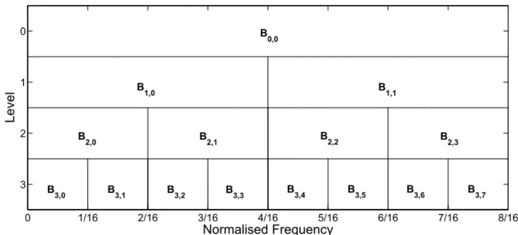
4.2.1 Partitioning of the Time-Frequency Domain . . . 54
4.2.2 Multivariate Frequency Partitioning - Examples . . . 56
4.3 Multivariate Time-Frequency Representation . . . 59
4.4 Simulations . . . 60
4.4.1 Sinusoidal Oscillation in Noise . . . 62
4.4.2 Amplitude and Frequency Modulated Signal Analysis . . . 63
4.4.3 Float Drift Data . . . 65
4.4.4 Doppler Speed Estimation . . . 65
4.4.5 Gait Analysis . . . 67
4.5 Multivariate Instantaneous Frequency Bias Analysis . . . 69
4.6 Summary . . . 71
Chapter 5. Phase Synchrony Spectrograms using Synchrosqueezing 72 5.1 Introduction . . . 72
Contents 7
5.3 Phase Synchronization using SST . . . 74
5.4 Simulations . . . 75
5.4.1 Synthetic signals . . . 76
5.4.2 Human motion analysis . . . 77
5.5 Summary . . . 78
Chapter 6. Automated Trading Using Phase Synchronization 79 6.1 Introduction . . . 79
6.2 Phase Synchrony and Algorithmic Trading . . . 80
6.2.1 Trading Algorithm Based Upon the Phase Synchrony of Assets . . . 81
6.3 Statistical Analysis of Phase Synchronization . . . 81
6.4 Simulations . . . 83
6.5 Summary . . . 86
Chapter 7. Multivariate Signal Denoising using Synchrosqueezing 87 7.1 Introduction . . . 87
7.2 Wavelet Denoising Techniques . . . 88
7.2.1 Univariate Wavelet Denoising . . . 88
7.2.2 Multivariate Wavelet Denoising . . . 89
7.3 Denoising using Multivariate Extension of Synchrosqueezing . . . 90
7.3.1 Denoising using Synchrosqueezing Techniques . . . 91
7.4 Simulations . . . 92
7.4.1 Denoising Sinusoidal Oscillations . . . 92
7.4.2 Denoising Frequency Modulated Oscillations . . . 95
7.4.3 Human Motion Denoising . . . 96
7.4.4 Float Drift Denoising . . . 97
7.4.5 Denoising in Motor Imagery BCI . . . 98
7.5 Summary . . . 100
Chapter 8. Bivariate and Trivariate EMD for Unbalanced Signals 101 8.1 Nonuniformly sampled BEMD . . . 102
8.1.1 Effect of Circularity on Direction Samples . . . 105
8.1.2 Simulation: Correlated Bivariate Data of Equal Channel Powers . . 106
8.1.3 Simulation: Noise Assisted Signal Decomposition . . . 107
8.1.4 Simulation: Speed Estimation using Doppler Radar . . . 109
8.2 Nonuniformly sampled Multivariate EMD . . . 109
8.2.1 Simulation: Noise Assisted Signal Decomposition . . . 112
8.3 Summary . . . 115
Chapter 9. Conclusion and Future Work 116 9.1 Conclusion . . . 116
9.2 Future Work . . . 118
9.2.1 Multivariate time and frequency partitioning . . . 118
9.2.2 Robust joint instantaneous frequency estimator . . . 119
9.2.3 Multivariate phase synchrony spectrograms . . . 119
9.2.4 Multivariate dynamically sampled EMD . . . 119
Bibliography 120 Appendix A. Implementation of Fourier Based Synchrosqueezing 130 A.0.5 STFT Implementation . . . 130
A.0.6 Instantaneous Frequency Estimation . . . 131
A.0.7 STFT Synchrosqueezing . . . 131
Appendix B. Multivariate Wigner Distribution 133
9
Statement of Originality
I declare that this is an original thesis and it is entirely based my own work. I acknowledge the sources in every instance where I used the ideas of other writers. This thesis was not and will not be submitted to any other university or institution for fulfilling the requirements of a degree.
List of Publications
To the best of my knowledge, the following are original works in which I have participated.
• Accepted Journal Publications
1. A. Ahrabian and D. P. Mandic, “A class of multivariate denoising algorithms based on synchrosqueezing,” IEEE transactions on Signal Processing, 2015 (to appear).
2. A. Ahrabian, D. Looney, L. Stankovic, and D. P. Mandic, “Synchrosqueezing-based time-frequency analysis of multivariate data,” Signal Processing, Vol. 106, pp. 331-341, 2015.
3. C. Park, D. Looney, N. U. Rehman, A. Ahrabian, and D. P. Mandic, “Classifi-cation of Mmotor imagery BCI using multivariate empirical mode decomposi-tion,” IEEE Transactions on Neural Systems and Rehabilitation Engineering,
Vol. 21, no. 1, pp. 10-22, 2013.
4. A. Ahrabian, N. U. Rehman, and D. P. Mandic, “Bivariate empirical mode decomposition for unbalanced real-world signals,” IEEE Signal Processing Let-ters, Vol. 20, no. 3, pp. 245-248, 2013.
5. A. Ahrabian, C. C. Took, and D. P. Mandic, “Algorithmic trading using phase synchronisation,” IEEE Journal of Selected Topics in Signal Processing, Vol. 6, no. 99, pp. 399-404, 2012.
0. List of Publications 11
• Accepted Conference Publications
1. A. Ahrabian and D. P. Mandic, “Estimation of phase synchrony using the synchrosqueezing transform,” IEEE International Conference on Acoustics, Speech and Signal Processing, pp. 759-763, 2014.
2. A. Ahrabian, D. Looney, F.A. Tobar, J. Hallatt, and D. P. Mandic, “Noise assisted multivariate empirical mode decomposition applied to Doppler radar data,” Sensor Signal Processing for Defence, p. 32, 2012.
List of Figures
2.1 The time-frequency resolution for both the STFT (upper panel) and CWT (lower panel) . . . 28 2.2 The Wigner distribution of a multicomponent signal, where the cross-term
is located in the region between the two auto-terms. (Source: [4]). . . 30 2.3 (Upper panel) The output of the ambiguity function, when processing a
multicomponent signal. It should be noted that the auto-terms are located near the origin of the figure, while the cross-terms are further away from the origin. (Lower panel) An illsutration of the kernel function being used to filter out (blue background) the cross-terms while retaining the auto-terms (white background). (Source: [4]). . . 32
3.1 Simulation showing the MEMD decomposition of the three channel syn-thetic signal, a(t), b(t), c(t). It can be seen from the simulation the modal alignment of the corresponding IMFs. This would not be achieved using the single channel EMD, to process the three channels independently. . . . 41 3.2 The time-frequency representations of both the wavelet based SST (upper
panel) and the CWT (lower panel), when processing a signal made from the addition of a linear frequency modulated oscillation and a sinusoidal oscillation. . . 44 3.3 The time-frequency representations of both the Fourier based SST (upper
panel) and the STFT (lower panel), when processing a signal made from the addition of a linear frequency modulated oscillation and a sinusoidal oscillation. . . 47
List of Figures 13
4.1 The partitioned frequency domain with the multivariate bandwidth given by Bls,ms, wherelscorresponds to the level of the frequency band, andms
is the frequency band index. . . 54 4.2 A comparison between the localization ratios B, for both the proposed
method and the MPWD, evaluated for a bivariate oscillation with the fol-lowing joint instantaneous frequencies: (upper panel) 10.5 Hz, (middle panel) 40.5 Hz, and (lower panel) 100.5 Hz. A window length of 1001 samples was used for the MPWD. . . 61 4.3 The time-frequency representations for both the proposed method (left
pan-els) and the MWPD (right panpan-els) for a bivariate AM/FM signal, with in-put SNR of (a) 10 dB, (b) 5 dB and (c) 0 dB. The window length used for MPWD was 681 samples. . . 64 4.4 Time-frequency analysis of real world float drift data. (a) The time domain
waveforms of bivariate float velocity data (b) The time-frequency represen-tation of float data using the proposed multivariate extension of the SST and (c) the MPWD algorithm. A window length 501 was used for the MPWD. . . 66 4.5 Time-frequency analysis of Doppler radar data. (a) The time domain
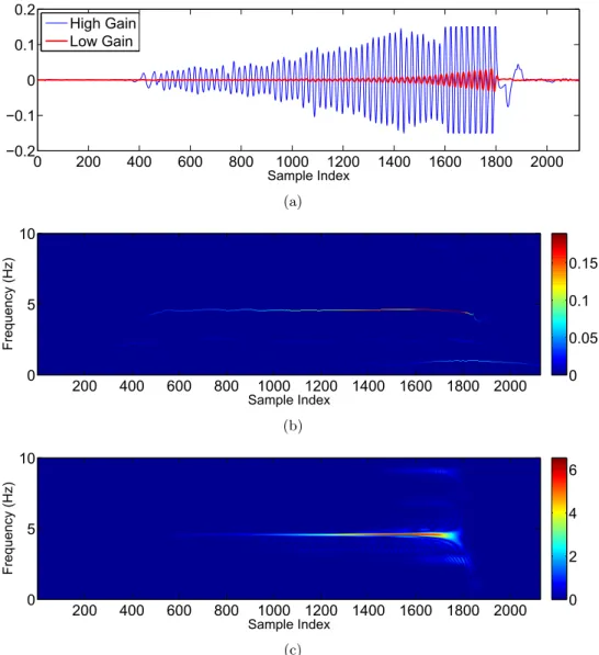
wave-forms of both the high gain and low gain Doppler radar data. (b) The time-frequency representation of Doppler radar data using the proposed multivariate extension of the SST and(c) the MPWD algorithm. A window length 1063 was used for the MPWD. . . 67 4.6 (a) The time domain representation of gait data obtained from the y-axis
of an acceleromter (left panel) and the time-frequency representation of the gait data using the channel-wise magnitude of the SST coefficients (right panel). (b) The multivariate extension of the SST (left panel) and the MPWD (right panel). A window length of 501 was used for the MPWD. . 68
5.1 Phase synchrony spectrograms of a bivariate linear chirp signal in white noise. (Upper panel) BEMD based phase synchrony method; (Lower panel) multivariate SST based phase synchrony method. . . 75
5.2 Phase synchrony in human walk. (a) Time domain representation of the accelerometer data. Phase synchrony spectrograms of the accelerometer data using (b) BEMD based phase synchrony method and (c) multivariate SST based phase synchrony method. . . 77
6.1 The outcome of the phase synchrony algorithm, with the indications for buying and selling for a window length of 800 trading days. (Top) The price of the leading asset Sainsburys. (Middle) The lagging asset Tesco with buy (solid vertical line) and sell (dashed vertical line) indicators. (Bottom) The volatility of Tesco. Graphs begin on 2003-05-05 and end on 2011-05-04. . . 84 6.2 The RoR of Phase Synchrony Algorithm (thick solid line), LMS
extrapo-lation (dashed) and MA crossover (thin solid line). Graphs begin on the 1000th trading day and end on 1500th trading day on Tesco stock. . . 85 6.3 The RoR of Phase Synchrony Algorithm (thick solid line), LMS
extrapo-lation (dashed) and MA crossover (thin solid line). Graphs begins on the 1000th trading day and end on 1500th trading day on Rolls-Royce stock. . . 85 6.4 The RoR of Phase Synchrony Algorithm (thick solid line), LMS
extrapo-lation (dashed) and MA crossover (thin solid line). Graphs begins on the 1000th trading day and end on 1500th trading day on Anglo-American stock. 86
7.1 Denoising of bivariate sinusoids. (a-c) (left panel) The reconstruction SNRs of the denoised signal of interest for both the proposed methods (MWSD and MFSD) and the standard MWD algorithm for bivariate sinusoidal oscil-lations in white Gaussian noise, and with equal channel SNRs. (a-c) (right panel) The reconstruction SNR for bivariate sinusoidal oscillations in noise using the MWSD algorithm. The blue line corresponds to the reconstruc-tion error for equal channel SNRs, while the red line corresponds to the reconstruction error for different channel SNRs. . . 93
List of Figures 15
7.2 The reconstruction SNRs of the bivariate FM signal in noise for both the proposed methods (MWSD and MFSD) and the MPW (upper panel). Com-parison of the proposed MWSD algorithm when processing a bivariate FM signal with equal (balanced) and different (unbalanced) inter-channel pow-ers (lower panel). . . 94 7.3 Time domain representation of the body motion accelerometer data,
per-taining to arm swings of a subject during walk. . . 95 7.4 Oceanographic float drift recordings. (a) The amplitude spectra of the
latitude and (b) the amplitude spectra of the longitude. . . 98 7.5 Ocean float denoising. (a) The denoised bivariate float using the proposed
MWSD method (left panel) and the MWD algorithm (right panel). (b) The amplitude spectra for both the MWSD and multivariate wavelet denoising algorithms for denoised signal corresponding to the latitude (left panel) and the longitude (right panel). . . 99 7.6 Motor imagery denoising. (a) The time-frequency representations of EEG
data pertaining to the left hand motor imagery, from the FC3 electrode (left panel) and T7 electrode (right panel). (b) The time-frequency repre-sentations of the denoised EEG signals using the MWSD algorithm, for the FC3 electrode (left panel) and T7 electrode (right panel). . . 100
8.1 Scatter plot for a bivariate signal, z=x+iy. (Left) A uniformly sampled unit circle (standard BEMD). (Right) A uniformly sampled ellipse, with higher density of samples along the major axis a(the proposed NS-BEMD). 102 8.2 The scatter plots (blue) and the 16 elliptically distributed projections (red)
for a bivariate signal with equal channel powers and varying channel corre-lations η. (a) η = 0, ǫ= 0.26, θ = 19.45o. (b) η = 0.3, ǫ= 0.52, θ= 43o. (c) η= 0.7,ǫ= 0.85, θ= 43.4o. (d)η= 0.9,ǫ= 0.95, θ= 45o. . . 104 8.3 The scatter plots (blue) and the 16 elliptically distributed projections (red)
for an uncorrelated bivariate signal of varying channel power ratio Ω. (a) Ω = 0.4,ǫ= 0.85,θ= 0.14o. (b) Ω = 0.16,ǫ= 0.98,θ= 0.04o. (c) Ω = 2.5,
8.4 The difference in reconstruction errors of the IMFs corresponding to tone
sin (7), for NS-BEMD and BEMD (∆ SNR), evaluated against the degree of correlation η and the number of projections k. . . 106 8.5 Reconstruction error (in SNR) in the IMFs for a two-tone signal in (8.9)
with varying channel power ratio, given by 10 log(Ω). (Top) Reconstruction using of the proposed NA-NSBEMD. (Bottom) Results of NA-BEMD. . . . 107 8.6 The time-frequency representation of the Doppler radar signal obtained via
NA-NSBEMD (top) and NA-BEMD (bottom) usingk= 8 projections. The noise channel power was 8 dB relative to the signal (10 log(Ω) = 8 dB). . . 108 8.7 Optional caption for list of figures . . . 110 8.8 Reconstruction error (in SNR) in the IMFs for a two-tone signal in (8.13)
with varying channel power ratio, given by 10 log(Ω). (Top) Reconstruc-tion of both the NA-NSTEMD and NA-MEMD algorithm for the 15 Hz tone. (Bottom) Reconstruction of both the NA-NSTEMD and NA-MEMD algorithm for the 10 Hz tone. Both algorithms used 32 samples. . . 113 8.9 Reconstruction error (in SNR) in the IMFs for a single tone sinusoidal
oscillation, using the proposed NS-TEMD and MEMD algorithms. Both algorithms used 32 samples. . . 114
17
List of Tables
4.1 Localization ratios, Bloc, for both the proposed algorithm and the MPWD. 64
5.1 The average synchrony, ρs, between the channels of a bivariate signal, at different frequency and noise levels. . . 76
6.1 Statistical verification of the phase synchronization between asset pairs us-ing the surrogate data generation method. The BEMD method for calcu-lating phase synchronization was used. . . 83 6.2 Percentage return on day 500 of the RoR graphs in Figs. 6.2-6.4 . . . 86
List of Abbreviations
AF: Ambiguity Function AM: Amplitude Modulation
BEMD: Bivariate Empirical Mode Decomposition CD: Cohen’s Class of Distribution
CWT: Continuous Wavelet Transform EEG: Electroencephalography
EMD: Empirical Mode Decomposition FT: Fourier Transform
fGn: fractional Gaussian noise FM: Frequency Modulation IMF: Intrinsic Mode Function
MEMD: Multivariate Empirical Mode Decomposition MWD: Multivariate Wigner Distribution
RM: Reassignment Method
STFT: Short Time Fourier Transform SST: Synchrosqueezing Transform
T-F: Time-Frequency WD: Wigner Distribution WGN: White Gaussian Noise
19
Chapter 1
Introduction
1.1
Background
The analysis and filtering of signal components from time series data is an important objective in signal processing. Traditionally Fourier based methods have used been used extensively for such tasks, where in particular applications have been found in commu-nication systems and filter design. However the underlying assumptions of linearity and time invariance of the time series are not guaranteed for many real world signals, where often both frequency and amplitude vary as a function of time. This has lead to the de-velopment of tools and techniques for the analysis of such signals, namely time-frequency algorithms.
Fourier analysis techniques have been widely utilized in analyzing the spectral con-tent of time series data. Fourier analysis initially emerged with the introduction of Fourier series, where a periodic signal is decomposed into a set of weighted sines and cosines, with frequencies given as integer multiples of a fundamental frequency, determined by the pe-riod of the signal being analyzed. By decomposing a pepe-riodic signal into a set of weighted harmonic trigonometric functions (basis functions), the basis functions provide a more convenient representation of the original periodic signal. The power of Fourier series anal-ysis arises due to the physical interpretation of the trigonometric basis functions. That is
a sine wave represents a pure oscillation of a physical system, such as the displacement of a vibrating mechanical system.
The Fourier series applies to a limited class of signals, namely periodic signals. As a result, the Fourier transform (FT) was developed in order to analyze aperiodic signals. An important application of the FT in signal processing is the decomposition of a signal into its frequency spectrum; where for a given frequency, the frequency spectrum provides information on both the amplitude and phase parameters of the corresponding sinusoidal basis function. It should be noted that, the Fourier transform requires that the input sig-nal being asig-nalyzed is both linear and time invariant (stationary1); where time invariance is
required due to the basis functions being sinusoidal oscillations of infinite duration, while the linearity assumption emerges as the Fourier transform linearly combines the sinusoidal oscillations with appropriate amplitudes (weights).
In order to address the limitations of Fourier analysis techniques in modelling time varying signals, the concept of the modulated oscillation was introduced in [1]; where both the amplitude and frequency of such oscillations vary as a function of time, and are respectively referred to as the instantaneous amplitude and frequency. This definition of frequency seems counterintuitive, as traditionally frequency is defined as the number of oscillations in a given time interval. However by imposing constraints on the definition of the instantaneous frequency, that is by assuming that the input signal is narrowband2 [2], or that the instantaneous frequency varies slowly [3], a physically meaningful description can be determined. The modulated oscillation model has found use in communication systems, that is, in the theory of amplitude modulated (AM) and frequency modulated (FM) systems [1]. In order to identify physically meaningful instantaneous amplitudes and frequencies for a given signal, techniques in time-frequency analysis have been employed. Time-frequency analysis techniques map a univariate signal onto a two dimensional surface, with each dimension measuring both time and frequency respectively. By an-alyzing a signal in the time-frequency domain, the time varying properties of an input signals oscillatory components is captured. The first of such algorithms was the short
1Stationarity is defined as the joint probability density function of the time series data being invariant with respect to time.
2
1.1 Background 21
time Fourier transform (STFT) introduced in [1], where the algorithm employs a sliding window function, in order to localize a signal in time where the Fourier transform is then applied, resulting in a time-frequency representation that captures the instantaneous fre-quency variation of a signals oscillatory components.
The STFT is fundamentally limited in resolving oscillations both in time and fre-quency [4]; implying that accurate localization along frefre-quency results in poor localization in time. Due to the STFTs constant window length, the resolution of the STFT is not dependent on frequency. For certain class of signals, i.e. transient signals and signals with spurious artifacts, a time-frequency algorithm with frequency dependent window length would provide a more physically meaningful time-frequency representation of the signal [5]. To this end, the continuous wavelet transform (CWT) was proposed as a variation of the STFT, where a frequency dependent scale factor was used to vary the window length.
Both the Fourier and wavelet based transforms, suffer from poor time and frequency localization. A class of algorithms that have been developed in order to overcome this problem are the quadratic time-frequency distributions [6], in particular the Wigner dis-tribution (WD) [7] [8]. Where the WD effectively calculates the Fourier transform of the instantaneous autocorrelation function, of the input signal. The Wigner distribution has been shown to perfectly localize a specific class of signals (namely linear frequency mod-ulated oscillations), however for multicomponent signals, the WD generates interference terms in the time-frequency domain that obscure the analysis of such signals.
More recently two radically different techniques have been proposed in order to gen-erate localized time-frequency representations; the first set of techniques are known as data driven algorithms, while the second set of algorithms are referred to as reassignment methods. The empirical mode decomposition (EMD) introduced the field of data driven time-frequency analysis and was developed by Huang et al. in [2]. The EMD decom-poses a signal into a set of narrowband oscillatory components termed, intrinsic mode functions (IMFs), where each IMF is determined via an iterated algorithmic procedure, thereby ensuring that the algorithm is fully data driven. The advantage of the EMD over conventional projection and quadratic based time-frequency algorithms is the adaptive nature of the algorithm, where the IMFs can be seen as a basis functions tailored to the
input signal. While the EMD has found applications in processing univariate time series data [9], the works in [10] identified the need for a multichannel extension of the EMD in order to effectively process multichannel interdependencies that arise in multivariate data. To that end, the complex extensions of the EMD were first introduced in the following works [11] [12] [13]; which ultimately led to the development of the multivariate EMD [14], a fully data driven multivariate time-frequency algorithm that has the capability of pro-cessing inter-channel interdependencies. It should be noted that, while the EMD and its multivariate extensions have been been applied to a wide range of data sets [15] [16] [17]; the underlying EMD algorithm still lacks solid mathematical description [18].
Finally, the concept of reassignment arose from the work by Kodera et al. [19] (re-formulations of the original reassignment method were also developed by [20]), where the time-frequency localization of the STFT was improved by using phase information in or-der to sharpen its time-frequency representation. While the original RM method proposed in [19] improved the localization of oscillatory components, a convenient inverse for the transform does not exist. More recently the work in [21] introduced a variation of the orig-inal RM, known as the synchrosqueezing transform (SST). Where the SST was origorig-inally developed as a post processing technique that was applied to the CWT, however unlike the techniques proposed in [19] [20], the SST is invertible, thus enabling the recovery of oscillatory components of interest.
1.2
Thesis Aims
This thesis primarily focuses on the following time-frequency algorithms, the chrosqueezing transform and multivariate extensions of the EMD. Where the syn-chrosqueezing transform has been shown to effectively generate time-frequency repre-sentations that localize signals with modulated oscillations that contain slowly varying instantaneous amplitudes and frequencies [3]; while multivariate extensions of the EMD have proved effective in analyzing the inter-channel dependencies that arise in multivariate data.
1.2 Thesis Aims 23
The routine recording of multivariate data has increasingly become commonplace in many disciplines of science and engineering, where such signals often contain time-varying oscillatory components. Accordingly, the need for signal analysis techniques for analyzing such data has been increasing, especially in the field of time-frequency analysis. To this end, the aims of this thesis can be stated as follows:
• Develop a multivariate extension of the synchrosqueezing transform, with applica-tions in multivariate time-frequency analysis, phase synchronization analysis, and multivariate signal denoising.
• Develop techniques to enhance the performance of multivariate extensions of the EMD, using nonuniform sampling techniques when processing data with power im-balances and inter-channel correlations.
A more detailed description of the thesis aims is provided in the following subsections.
1.2.1 Multivariate extension of SST
This thesis first seeks to introduce a multivariate extension of the synchrosqueezing trans-form, by identifying a set of modulated multivariate oscillations using a multivariate ex-tension of a frequency partitioning algorithm first introduced in [22]. Recently the notion of the multivariate modulated oscillation was introduced in [23], where multivariate time series data are modeled as a single oscillatory structure with a common instantaneous am-plitude and frequency. This thesis then develops a multivariate time-frequency representa-tion using the synchrosqueezing transform, such that multivariate modulated oscillarepresenta-tions can be identified.
Phase synchronization has emerged as an important concept in quantifying interac-tions between two oscillatory systems. More recently phase synchrony spectrograms have been developed by [24] [25], where the time and frequency variations of the interdepen-dencies between oscillatory components can be visualized. This thesis seeks to develop a phase synchrony spectrogram using the multivariate extension of the SST. Furthermore an automated trading system using phase synchronization and the SST is also developed,
where it is demonstrated that the interdependencies that arise between two stock prices can be exploited in order to develop a trading algorithm.
Finally, conventional signal denoising algorithms using thresholding [26] are based on the discrete wavelet transform (DWT) and more recently the EMD [27] [28]. However, DWT based denoising methods suffer from limited time and frequency resolution; while EMD based signal denoising methods are inherently limited by the EMDs lack of solid theoretical foundation. In order to overcome these limitations recently an SST based de-noising technique has been proposed in [29]; however this caters only for univariate time series data. To this end, this thesis also seeks to develop a multivariate signal denoising algorithm using the proposed multivariate extension of the SST.
1.2.2 Nonuniformly sampled multivariate extension of EMD
Both the bivariate and corresponding multivariate EMD algorithms employ a uniform sampling scheme that projects a bivariate/multivariate signal across multiple direction in order to estimate the local mean. This thesis seeks to show that for bivariate/multivariate signals with power imbalances and inter-channel correlations, that the use of a nonuniform sampling scheme would yield a performance improvement over existing uniformly sampled bivariate/multivariate EMD algorithms.
1.3
Original Contributions
A description of the contributions of this thesis are now presented:
1. Multivariate extension of the SST: Given a multivariate signal, the proposed multivariate extension of the SST seeks to identify a set of matched monocomponent signals that is common to the multivariate data, by partitioning along frequency, the time-frequency domain.
2. Multivariate Time-Frequency Representation: A multivariate time-frequency representation is introduced using the multivariate extension of the SST, such that a
1.4 Thesis Outline 25
single time-frequency representation is determined that best captures the oscillatory dynamics of the multivariate data.
3. Phase Synchrony Spectrogram: Using the SST, a phase synchrony estimation technique is developed so as to capture both time and frequency variations of phase synchronization.
4. Algorithmic trading using phase synchrony: A systematic trading algorithm using the synchrosqueezing transform and phase synchrony is developed.
5. Multivariate signal denoising using the SST: A multivariate signal denoising technique using the multivariate extension of the SST is developed, along with a multivariate extension of thresholding.
6. Nonuniformly sampled EMD algorithms: A nonuniform projection scheme that is dependent upon the signal statistics is developed for both the bivariate and multivariate EMD algorithms.
1.4
Thesis Outline
The organization of this thesis is as follows: Chapter 2 provides a review of conventional linear and quadratic time-frequency algorithms, with specific focus on the STFT, CWT, Wigner distribution and Cohen’s class of distributions; moreover Chapter 2 also provides a review on the modulated oscillation model. In Chapter 3, the primary focus is on time-frequency algorithms that have been recently proposed in order to enhance the resolution of oscillatory features over the methods introduced in Chapter 2; where these methods include both data driven methods, such as the EMD, and reassignment methods such as the SST.
Chapter 4 introduces the multivariate extension of the synchrosqueezing transform, and by using the concept of joint instantaneous frequency for multivariate data, an applica-tion is developed in multivariate time-frequency analysis. The advantages of the proposed multivariate time-frequency representation is illustrated on both synthetic and real world
data. For rigor, an error bound which evaluates the accuracy of the multivariate instan-taneous frequency estimator is also provided.
Chapter 5 introduces a phase synchrony spectrogram using the multivariate extension of the synchrosqueezing transform (first presented in Chapter 2). The chapter introduces the definition of phase synchronization, before introducing the proposed method. Simu-lations both on synthetic and real world data illustrate the performance of the proposed method.
Chapter 6 presents a systematic trading algorithm using both the synchrosqueezing transform and phase synchronization. Where the chapter first introduces the concept of lead-lag relationship between two stocks, before introducing the proposed trading system using phase synchrony and the SST. Simulations are conducted on real world stock prices. In Chapter 7 a multivariate signal denoising algorithm is presented, using the mul-tivariate extension of the synchrosqueezing transform introduced in Chapter 2, where a multivariate threshold is then introduced in order to remove noise components, while retaining signal components of interest. The performance of the proposed multivariate denoising algorithm is illustrated on both synthetic data and real world data.
Chapter 8 introduces the nonuniformly sampled bivariate and trivariate EMD al-gorithms, where the objective is to determine optimal projection directions, such that accurate estimation of the local mean is carried out when processing data with power imbalances and inter-channel correlations. Finally, the conclusions and future work for this thesis are presented in Chapter 9.
27
Chapter 2
Linear and Quadratic
Time-Frequency Representations
This chapter first provides an overview of Fourier analysis methods and the modulated oscillation model. The chapter then provides an overview of both linear and quadratic time-frequency methods.
2.1
Fourier Analysis
Given a periodic signalx(t) with periodT, such that the following condition is satisfied
x(t+zT) =x(t) z∈Z, (2.1)
then (2.1) can be represented by a sum of complex periodic sinusoidal oscillations that are scaled by some appropriate parameter anz, such that the periodic signal x(t) can be
represented by the following
x(t) = X nz∈Z anze ˙ ı2πnz t T . (2.2)
It should be noted that, in the Fourier series analysis of periodic signals, the periodic complex sinusoidal oscillations are harmonics of the fundamental frequency, fo = T1. In order to identify the parameter anz, first note that the inner product between any two
sinusoidal oscillations of differing frequency is equal to zero, that is
D e˙ı2πmz tT , e ˙ ı2πnz t T E = Z T 2 −T 2 eı˙2πmz tT e− ˙ ı2πnz t T dt= 0, (2.3)
when mz 6= nz. Accordingly, by calculating the inner product of a sinusoidal oscillation for a given indexnz with the original signal x(t), the coefficients anz of the Fourier series
can be determined anz = 1 T Z T 2 −T 2 x(t)e−˙ı2πnz tT dt. (2.4)
The Fourier transform extends the Fourier series (that analyzes periodic signals) to the analysis of aperiodic signals. This is achieved by taking the periodT of the normalised Fourier series coefficients to infinity (T → ∞) thereby allowing the analysis of aperiodic signals, that is X(ω) = lim T→∞XnzT = limT→∞ Z T 2 −T 2 x(t)e−˙ı2πnz tT dt= Z ∞ −∞ x(t)e−ıωt˙ dt. (2.5) with 2Tπ =δω → ω and 2Tπ = ω. The term X(ω) corresponds to the Fourier coefficients that captures both amplitude and phase information from the signal x(t), for a given fre-quencyω. The amplitude spectrumA(ω) =|X(ω)|, contains information pertaining to the magnitude of the sinusoidal oscillations for a given frequencyω, while the phase spectrum Φ(ω) = ∠X(ω) (where ∠ corresponds to the angle of a complex number), captures the time distribution of the sinusoidal oscillations. Both the Fourier transform and Fourier series methods, assume that the amplitude and phase of the sinusoidal basis functions are time-invariant. However, for many real world signals this assumption is invalid. To this end, the modulated oscillation model introduced in the section that follows seeks to overcome this modeling problem.
2.2 Modulated Oscillations 29
2.2
Modulated Oscillations
Consider a signal where both the amplitude and phase are a function of time, such that the signal can be represented by the following model [1] [30],
x(t) =a(t) cosφ(t) (2.6)
where a(t) and φ(t) are respectively the instantaneous amplitude and phase (where the derivative of the instantaneous phase results in the instantaneous frequency φ′(t)). Such signals, referred to as modulated oscillations (where the model (2.6) has both an amplitude modulated term, and frequency/phase modulated term) arise in many real world scenarios and applications; for example in communication systems the modulation of the message signal with either the amplitude and frequency of a carrier is used to transmit information. In Fourier theory, it is assumed that, a(t) = ˆaand φ(t) = ˆφt, where ˆaand ˆφare constant; implying that the underlying signal being analyzed is stationary with respect to the am-plitude and phase. However it should be noted that, many real world signals, such as data obtained in seismology, have time-varying signal [31] characteristics that are better mod-eled by assuming time-varying instantaneous phases and amplitudes. However, while the potential advantages of modeling oscillations in terms of (2.6) are apparent, identifying the instantaneous amplitude and phase for a given signal is a non trivial task [30]. This can be illustrated by the following example: given an amplitude modulated signal, xAM(t) with instantaneous amplitude aAM(t) = 2sin(ωt), and instantaneous phase φAM(t) = ωt, the equivalent frequency modulated representation xF M(t) = xAM(t), has an instantaneous amplitude, xF M(t) = 1 and instantaneous phaseφF M(t) = 2ωt; implying that identifying a unique pair of instantaneous amplitudes and phases for a given signal x(t) is not well defined.
In order to overcome this problem, the works in [1, 8, 32–34] applied the Hilbert transform to the signal x(t), so as to generate a complex representation known as the analytic signal x+(t), given by
x+(t) =a(t)eıφ˙ (t) =x(t) + ˙ıH{x(t)} (2.7)
where H{·} is the Hilbert transform operator, and ˙ı = √−1. Given that the Hilbert
transform has been applied to a product of two functions; that is the instantaneous am-plitude and phase (shown in (2.6)), the work in [35] derived constraints on the amam-plitude spectra of the respective functions. That is the spectra for both the instantaneous phase and amplitude must be nonoverlapping [36]. The analytic signal x+(t) is complex valued
and admits a unique time-frequency representation for the signalx(t), based on the deriva-tive of the instantaneous phase,φ(t). It should be noted that, while applying the Hilbert transform yields a unique instantaneous amplitude and frequency, the physical interpre-tation of such quantities is not always apparent for many real world signals; that is if the instantaneous frequency is rapidly changing, then obtaining useful information pertaining to the underlying process is limited. As an example, the instantaneous frequency and amplitude of a broad band signal (e.g. white Gaussian noise) would yield instantaneous frequency and amplitude estimates that vary rapidly with time, and would have not have an intuitive physical explanation. As a result, identifying the instantaneous amplitude and frequency terms is primarily limited to narrowband signals, where the instantaneous frequency and amplitude vary slowly. This can be illustrated by considering the global moments of the instantaneous frequency and bandwidth, in relation to the global moments of the frequency spectrum of the signal of interest. The global mean frequency of both the instantaneous frequency ωx(t) = φ
′
(t), and the analytic frequency spectrum X+(ω),
is given by ωx= 1 E Z ∞ −∞| x+(t)|2ωx(t) dt, (2.8) ωx= 1 E Z ∞ 0 ω|X+(ω)|2dω, (2.9)
where the global mean frequency, is effectively the average frequency present in the signal
x+(t) and E is the total energy of the Fourier coefficients given by
E= 1 2π
Z ∞
0 |
2.2 Modulated Oscillations 31
In order to quantify the spread of frequency around the global mean frequency, the global second momentσ2x needs to be determined, and is given by
σ2x= 1 E Z ∞ −∞| x+(t)|2σ2x(t) dt, (2.11) σ2x= 1 E Z ∞ 0 (ω−ωx)2|X+(ω)|2dω, (2.12) where σ2
x(t) is the instantaneous second central moment, and is given by
σx2(t) = | d
dtx+(t)−ıω˙ xx+(t)| |x+(t)2|
, (2.13)
where the instantaneous second central moment effectively captures the variation of the instantaneous frequency around the mean frequency as well as capturing the rate of change of amplitude modulation; this can be illustrated rewriting the instantaneous second central moment as
σx2(t) = (ωx(t)−ω)2+υ2x(t), (2.14) where υx(t) is the instantaneous bandwidth, and is defined as υx(t) =a′(t)/a(t).
Given an analytic broadband signalxb(t) from (2.12), observe that the global second moment would be large, implying a significant amount of frequency deviation around the global mean frequency. Given a large global second moment, from (2.11) the instantaneous second central moment would also need to be large; if a′(t) is assumed to be low (that is a slowly varying instantaneous amplitude), then from (2.14) it can be seen that the variation of the instantaneous frequency around the global mean frequency would need to be large, implying that broadband signals would yield rapidly changing instantaneous frequency estimates. Furthermore, the modulated oscillation model when representing multicomponent signals has a difficult physical interpretation that is addressed in the following section.
2.2.1 Multicomponent Modulated Oscillations
A multicomponent signal is defined as follows
x+(t) = Nm X nm=1 anm(t)e ˙ ıφnm(t), (2.15)
where each component indexed by nm, has an instantaneous frequency φ′nm(t) that is
narrowband. The physical interpretation of the instantaneous frequency for a multicom-ponent signal can lead to unusual results. To illustrate this, consider a two-commulticom-ponent signal x(t) = a1eıω˙ 1t+a2eıω˙ 2t, the instantaneous frequency φ
′ (t) and amplitude a(t) is given by [37–39] φ′(t) = 1 2(ω1+ω2) + 1 2(ω2−ω1) a22−a21 a2(t) , (2.16)
with instantaneous amplitude
a(t) =a21+a22+ 2a21a22cos(ω2−ω1)t, (2.17)
where it should be observed from (2.16) that the instantaneous frequency of the multi-component signal is the average of the two separate frequencies (ω1 andω2) whena1 =a2,
that is the signal components are balanced in power. If a1 6= a2, then the estimated
instantaneous frequency has an oscillatory component, that implies the signal x(t) is fre-quency modulated as well as amplitude modulated. Moreover the estimated instantaneous frequencyφ′(t) can vary beyond the range ofω1 and ω2, which has no convenient physical
interpretation.
To this end, in order to estimate the instantaneous frequency of a multicomponent sig-nal, a time-frequency or signal decomposition (e.g. band pass filter) algorithm is required in order to isolate the individual monocomponent signals that exist in the multicomponent signal, so as to estimate physically meaningful instantaneous frequencies. Furthermore, to obtain physically meaningful estimates of the instantaneous frequency for multicomponent signals, the work in [37] demonstrated that the weighted average instantaneous frequency
2.3 Linear Time-Frequency Representations 33 estimator, given by φ′W A(t) = PNm nm=1a 2 nm(t)φ ′ nm(t) PNm nm=1a 2 nm(t) , (2.18)
provides a physically meaningful interpretation of the instantaneous frequency, as the power weighted average of the instantaneous frequencies of the monocomponent oscilla-tions.
2.3
Linear Time-Frequency Representations
2.3.1 Short-Time Fourier Transform
The identification of modulated oscillations of the form (2.6), require a class of algorithms known as time-frequency methods; that is the frequency content of the signal is determined at each point in time. The Fourier transform assumes that the frequency components in the signal x(t) are stationary. In order to analyze the frequency components along time, the short time Fourier transform (STFT) was introduced [1], that applies a sliding window functionw(t), to the signal and then calculates the Fourier transform, that is
S(τ, ω) = Z ∞
−∞
w(t−τ)x(t)e−ıωt˙ dt, (2.19) whereS(τ, ω) corresponds to the STFT coefficients; with the corresponding inverse of the STFT given by x(t) = 1 2πw(t−τ) Z ∞ −∞ S(τ, ω)eıωt˙ dω, (2.20) The STFT is fundamentally limited in simultaneously resolving signal components both in time and frequency. This is due to the uncertainty principle in signal processing that states the following [4]
σ2tσ2ω≥ 1
4, (2.21)
where σ2
t is defined as the duration of a signal in time (for this particular example the duration of the window function is measured), and σω2 corresponds to the duration of the
window function in the frequency domain, that is σ2t = R∞ −∞τ2|w(τ)|dτ R∞ −∞|w(τ)|dτ , σ2ω= R∞ −∞ω2|Fw(ω)|dω R∞ −∞|Fw(ω)|dω ,
where Fw(ω) is the Fourier transform of the window function. Intuitively, (2.21) implies that in order to achieve a high frequency localization (that is small frequency duration), a window with a long duration (by extension a long window length) needs to be selected, while in order to achieve a high time localization a window with a small duration needs to be selected while leading to lower frequency localization. The short-time Fourier transform has been the de-facto standard for analyzing the oscillatory components of nonstationary signals, with applications in geophysics [40] and bioengineering [41].
2.3.2 Continuous Wavelet Transform
The continuous wavelet transform [5] is a projection based time-frequency algorithm that identifies oscillatory components of interest through a series of localized time-frequency filters known as wavelets. A wavelet ψ(t) is a finite oscillatory function, which when convolved with a signal x(t), in the form
W(as, b) = Z a−s1/2ψ∗ t−b as x(t)dt, (2.22)
whereW(as, b) are the wavelet coefficients. The waveletψ(t) is a square integrable function that satisfies the admissibility condition
Z R
|ψˆ(ξ)|2
ξ dξ <∞ (2.23)
where ˆψ(ξ) is the Fourier transform of the mother wavelet ψ(t). For each scale-time pair (as, b), the wavelet coefficients in (2.22) and can be seen as the outputs of a set of scaled
2.3 Linear Time-Frequency Representations 35
Time
Frequency
Time
Frequency
Figure 2.1: The time-frequency resolution for both the STFT (upper panel) and CWT (lower panel) .
bandpass filters. The scale factor as shifts the bandpass filters in the frequency domain, and also changes the bandwidth of the bandpass filters.
It should be noted that, the STFT has a constant time and frequency resolution for both low and high frequencies, as illustrated by Fig. 2.1 (upper panel). Where the continuous wavelet transform can be seen as a variation of the STFT, where the length of the window is varied as a function of frequency (shown in Fig. 2.1 (lower panel)). Accordingly, the CWT has high time resolution and low frequency resolution at high frequencies, while at low frequencies the time resolution is low and the frequency resolution is high. This is particularly useful for the analysis of transient oscillations, where it is important to localize the oscillation along time. The continuous wavelet transform has been applied to a wide range of problem ranging from geophysical [42] and biomedical
engineering [43] to gear box fault detection [44].
2.4
Quadratic Time-Frequency Representations
Quadratic time-frequency distributions (QTFD) generate time-frequency representations of a signal, by mapping the energy of the original signal to the time and frequency domain. The quadratic time-frequency representation Q(t, ω) of a signal x(t) need to satisfy the following [4], so as to be considered a QTFD:
1. The energy condition
E = 1 2π Z ∞ −∞ Z ∞ −∞ Q(t, ω)dt dω, (2.24)
where E is the energy of the signalx(t).
2. The frequency marginal condition
|X(ω)|2= Z ∞
−∞
Q(t, ω)dt, (2.25)
where X(ω) is the Fourier transform of the signal x(t).
3. The time marginal condition
|x(t)|2 = 1 2π Z ∞ −∞ Q(t, ω)dω. (2.26) 2.4.1 Wigner Distribution
The Wigner distribution (WD) function [7] [8] [45] is defined as the Fourier transform of the local/nonstationary autocorrelation function Rc(t, τ) =x(t+τ /2)x∗(t−τ /2), and is given by the following
W D(t, ω) = Z ∞
−∞
2.4 Quadratic Time-Frequency Representations 37 Time Frequency Auto−term Auto−term Cross−term
Figure 2.2: The Wigner distribution of a multicomponent signal, where the cross-term is located in the region between the two auto-terms. (Source: [4]).
where the Wigner distribution satisfies the properties shown in (2.24)-(2.26) [4]. Where the localization properties of the WD can be illustrated by the following example: consider a linear frequency modulated oscillation,x(t) =Aeı˙(ω0t+k2t2), where the WD is determined
as follows W Dx(t, ω) =A2 Z ∞ −∞ eı˙(ω0(t+τ /2)+k2(t+τ /2)2)e−ı˙(ω0(t−τ /2)+k2(t−τ /2)2)e−ıωτ˙ dτ =A2 Z ∞ −∞ eı˙(ω0τ+ktτ)e−ıωτ˙ dτ =A2δ(ω−(ω0+kt)), (2.28)
where it can be observed that the Wigner distribution localizes the energy of the signal along the instantaneous frequency curve, φ′(t) = ω0 +kt, of the linear frequency
mod-ulated signal, while the STFT and CWT would spread the energy of the signal around the vicinity of the instantaneous frequency curve. While the WD perfectly localizes the energy of linear frequency modulated oscillations, for FM signals that contain higher order polynomial terms the Wigner distribution introduces interference terms that deviate from the instantaneous frequency curves of the signal [4]. The instantaneous frequency of a modulated oscillation of the form (2.7), is defined as the normalized first moment of the
Wigner distribution with respect to frequency, that is φ′(t) = R∞ −∞ωW D(t, ω)dω R∞ −∞W D(t, ω)dω , (2.29)
where the instantaneous frequency is effectively defined as the average frequency present at each time point [46]. It should be noted that, the performance of the WD reduces for multicomponent signals, where this can be demonstrated by the following multicomponent signal, x(t) =Aeı˙(ω1t+k2t2) +Aeı˙(ω2t+k2t2), where ω
1 > ω2, and the Wigner distribution is
given by W Dx(t, ω) =A2 Z ∞ −∞ e˙ı(ω1(t+τ /2)+k2(t+τ /2)2) +eı˙(ω2(t+τ /2)+k2(t+τ /2)2) ×e−˙ı(ω1(t−τ /2)+k2(t−τ /2)2) +e−˙ı(ω2(t−τ /2)+k2(t−τ /2)2)e−˙ıωτ dτ =A2δ(ω−(ω1+kt)) | {z } auto−term +A2δ(ω−(ω2+kt)) | {z } auto−term +A2δ(ω−(1 2(ω1+ω2) +kt))cos(ω2−ω1)t | {z } cross−term . (2.30)
From (2.30), the terms corresponding to the instantaneous frequency curves of the separate monocomponent signals are known as the auto-terms, while the interference between the two monocomponent signals yields a third term in (2.30) known as the cross-term. It should be noted that the instantaneous frequency of the cross-term is bounded between the auto-terms, thereby making the suppression of such terms difficult. Fig. 2.2 illustrates the effect of the cross-term when processing a two-component signal.
2.4.2 Cohen Class of Distributions
In order to reduce the effects of the cross-terms introduced by the standard Wigner distri-bution when processing multicomponent signals1, the Cohen’s class of distributions (CD) were introduced in [6] [47]. Before introducing the Cohen’s class of time frequency
rep-1
It should be noted that, other techniques such as the pseudo WD and smoothed WD also suppress cross-terms [4].
2.4 Quadratic Time-Frequency Representations 39 0 0 Delay time Shift Frequency Cross−term Auto−term Cross−term 0 0 Delay time Shift Frequency Auto−term Cross−term Cross−term
Filtered Out Components
Figure 2.3: (Upper panel) The output of the ambiguity function, when processing a mul-ticomponent signal. It should be noted that the auto-terms are located near the origin of the figure, while the cross-terms are further away from the origin. (Lower panel) An ill-sutration of the kernel function being used to filter out (blue background) the cross-terms while retaining the auto-terms (white background). (Source: [4]).
resentations, an explanation of the ambiguity function (AF), shall be given. Where the ambiguity function is defined as
AF(t, ω) = Z ∞
−∞
x(t+τ /2)x∗(t−τ /2)e−ıωt˙ dt, (2.31) and is critical for suppressing cross-terms while preserving the auto-terms [48] [49]. The ambiguity function is related to the Wigner distribution via the application of the two dimensional Fourier transform (see [4] for details). Fig. 2.3 illustrates the primary differ-ence between the WD and the AF, where the ambiguity function has auto-terms located near the origin, with the cross-terms populating the regions around the auto-terms. As a
result, a functionc(τ,Φ) termed the kernel is applied to the ambiguity function such that the regions where the cross-terms are present are filtered while preserving the regions con-taining the auto-terms. The two dimensional Fourier transform of the resulting ‘filtered’ ambiguity function is then carried out in order to generate the appropriate time-frequency representation. The CD of a signal is given by
CW D(t, ω) = 1 2 Z ∞ −∞ c(τ,Φ)AF(τ,Φ)eı˙Φte−˙ıωτ dτ dΦ. (2.32) It should be noted that, while using the above procedure reduces the effects of the cross-terms, the localization of the auto-terms is also reduced. Finally, the Cohen’s class of distributions can be seen as the two dimensional smoothing of the WD; where the kernel function is effectively behaving as a low pass filter.
41
Chapter 3
Localized Time-Frequency
Representations
In this chapter an overview is provided of data driven and reassignment based time-frequency algorithms. Where the objective is to generate time-time-frequency representations that overcome the tradeoff that exists between the time and frequency resolution in con-ventional linear and quadratic time-frequency (T-F) algorithms.
3.1
Data Driven Time-Frequency Analysis
Data driven time-frequency methods have emerged as an important class of techniques for generating highly localized time-frequency representations. In this section an overview of the data driven time-frequency algorithms is presented starting with the empirical mode decomposition, and then presenting the corresponding multivariate extensions.
3.1.1 Empirical Mode Decomposition
Due to the uncertainty principle projection based time-frequency methods are inherently limited in resolving signal components both in time and frequency. In order to resolve this limitation a novel signal decomposition algorithm has been proposed [2] termed the empirical mode decomposition (EMD); where the objective is to decompose a signal into a set of amplitude and frequency modulated components termed intrinsic mode functions (IMFs). In order for a signal component to be considered as an IMF, there are two conditions that need to be satisfied, where the first condition is that the number of zero crossing and local extrema must be equal or at most differ by one, and the second condition is that the mean of the interpolated local maxima and local minima must be approximately equal to zero. The IMFs are calculated algorithmically by the sifting process [50], which is outlined in Algorithm 1.
Algorithm 1 Empirical Mode Decomposition (EMD) 1. Let ˆx(t) =x(t), where x(t) is the original signal 2. Identify all the local maxima and minima of ˆx(t).
3. Find a lower ‘envelope’, el(t) that uses a cubic spline interpolation in order to locate all of the minima points.
4. Find a upper ‘envelope’,eu(t) that uses a cubic spline interpolation in order to locate all of the maxima points.
5. Next the local mean is calculated according to the equationm(t) = (el(t) +eu(t))/2. 6. Subtract the local mean value from ˆx(t), d(t) = ˆx(t)−m(t) (nis an order of IMF). 7. Let ˆx(t) = d(t) and repeat the above process from step 2); until d(t) becomes an
IMF.
Given a set of finite IMF decompositions, the reconstruction of the original signal
x(t) is given by x(t) = Ni X ni=1 Γni(t) +r(t) (3.1)
where Γni(t) with ni = 1, . . . , Ni, is the set if IMFs and r(t) is the residue. Due to the
3.1 Data Driven Time-Frequency Analysis 43
IMFs in order to obtain a time-frequency estimate of the original signal. The Hilbert transform of an IMF, Γni(t) is given by
H{Γn i(t)}= Pc π Z ∞ −∞ Γni(t′) t−t′ dt′ (3.2)
where Pc is the Cauchy principal value. The resulting analytic signal is given by
x+(t) = Ni X ni=1 Γni(t) + ˙ıH{Γni(t)}= Ni X ni=1 ani(t)e ˙ ıθni(t) (3.3)
where ani(t) and θni(t) denote the instantaneous amplitude and phase respectively, for a
given IMF index ni. Given the instantaneous phase, the instantaneous frequency ωni(t)
for each IMF can then be determined1. Accordingly, given an instantaneous frequency estimate for each IMF at each time instant, a time-frequency representation E(t, ω) can then be generated, as follows
E(t, ω) =ani(t)δ(ω−ωni(t)) ni,= 1, . . . , Ni (3.4)
where δ(·) is the delta function.
The EMD has found a number of successful applications ranging from the biomedical signal processing [9] [52], to seismic data analysis [53], where in particular researchers di-rectly exploit the IMFs in order to carry out data analysis. Empirical mode decomposition is particularly useful in analyzing signals, where conventional basis functions of both the Fourier and wavelet transforms are not well suited; as an example in image processing where the signals are discontinuous and are not smoothly varying [10]. In [54], the EMD has been shown to behave as a dyadic filter bank, when processing broadband noise pro-cesses.
Due to the data adaptive nature of the EMD, its application to multichannel data would yield IMFs that, 1) are different, in terms of the number IMFs and the oscillatory
1It should be noted that there are a number of techniques in order to estimate the instantaneous frequency in the EMD framework. Some of these methods are outlined in [51].
dynamics for a given IMF index across channel, 2) the mode mixing phenomena; where similar modes appear across multiple IMFs, which further impedes multichannel data analysis using univariate EMD [10]. A potential solution to the mode mixing problem was introduced in [55], where a variation of the univariate EMD algorithm was proposed known as the ensemble empirical mode decomposition (EEMD). This was achieved by first adding white Gaussian noise (WGN) to the signal x(t), and then applying EMD. This process is then repeated for different white Gaussian noise realizations, and the re-sulting IMFs of the same index are averaged yielding IMFs that are well separated in frequency (i.e. reduction in the mode mixing effect). It should be noted that the EEMD is computationally expensive, as the number of realizations that need to be simulated is large; and the EEMD does guarantee that for multichannel data, for a given IMF index as having similar oscillatory dynamics across channel. To this end, a number of multichannel extensions of the EMD have been proposed in order to overcome this problem.
3.1.2 Bivariate Empirical Mode Decomposition
For the case of bivariate (or complex valued) data, several extensions of EMD have been recently proposed: 1) Complex EMD by Tanaka and Mandic [11], 2) rotation- invariant EMD by Altaf et al. [12], and 3) bivariate EMD by Rilling et al. [13].
Complex EMD (CEMD) applies standard univariate EMD separately to the real and imaginary data channels, thus not guaranteeing the same number of IMFs across data channels, which is a major requirement in real-world applications. The rotation-invariant EMD (RI-EMD) is a fully bivariate (complex) extension of EMD, which operates by taking projections of the bivariate input signal along two directions in the complex plane to compute the local mean. The bivariate signal envelopes are calculated by interpolating the envelopes of those univariate (real-valued) projections, and the local mean of a complex signal is determined by taking the mean of the envelopes. Although the RI-EMD gives the same number of IMFs for both the signal components, it is not well-equipped to deal with fast signal dynamics due to a low number of signal projections, which limits its practical usefulness.
3.1 Data Driven Time-Frequency Analysis 45
To alleviate these problems, Rilling et al. [13] proposed an algorithm that operates by first projecting an input bivariate signal in Nk uniformly spaced directions along a unit circle. The extrema points of such multiple real-valued univariate projections are calculated separately, while the interpolation of such extrema results in bivariate envelopes, one for for each direction. The sifting process is thus carried out according to conventional EMD. Algorithm 2 shows the steps required for calculating the local mean of a bivariate signal in BEMD [13]. The BEMD algorithm has found a range applications ranging from phase synchrony analysis [10] [56], to fault detection in aircraft components [57] and EEG data analysis [41].
Algorithm 2: Bivariate Empirical Mode Decomposition 1. Given a set of directions φnk =
2πnk
Nk , where nk = 1, . . . , Nk project the complex
valued signal xc(t) along the directionsφnk:
pφnk(t) =Re
ejφnkxc(t) (3.5)
2. Extract the locations tnk
i of the extrema points of pφnk(t). 3. Interpolate the set (tnk
i , xc(tnik)) to obtain the envelope curveeφnk(t) in the direction
φnk.
4. Compute the mean of all envelope curves:
m(t) = 1
Nk X
nk
eφnk(t) (3.6)
5. Subtract m(t) from the input signal in order to obtain the oscillatory component
d(t).
3.1.3 Multivariate Empirical Mode Decomposition
The BEMD algorithm provided an intuitive extension of the empirical mode decomposition so as to process bivariate oscillations. Where in the bivariate example, the oscillations are viewed as rotations where faster rotating components contain high frequency oscillations in each separate channel, and slower rotations correspond to low frequency oscillations in each channel.
Algorithm 3 Multivariate Empirical Mode Decomposition (MEMD) 1. Choose a suitable pointset for sampling on an (n-1) hypersphere. 2. Calculate a projection, denoted by pθk(t)Tt
t=1, of the input signal x(t)Tt=1t along the
direction vector uθk, for all k (the whole set of direction vectors), giving pθk(t)T
t=1 as
the set of projections 3. Find the time instantstθk
i corresponding to the maxima of the set of projected signals
pθk(t)Tt
t=1
4. Interpolate [tθk
i ,x(t θk
i )] to obtain multivariate envelope curves eθk(t)Kk=1.
5. For a set of K direction vectors, the mean m(t) of the envelope curves is calculated as m(t) = 1 K K X k=1 eθk(t) (3.7)
6. Extract the ’detail’ d(t) using d(t) = x(t)−m(t). If the ’detail’ d(t) fulfills the stoppage criterion for a multivariate IMF, apply the above procedure to x(t)−d(t), otherwise apply it tod(t)
Inspired by the BEMD, the work in [58] developed a trivariate extension of the EMD algorithm. The algorithm first models the trivariate signal as a pure quaternion2, where the signal is then projected along multiple directions across a three dimensional sphere (the directions selected across the sphere are along the equi-longitudinal lines). The en-velopes and corresponding local mean are then determined (using the principles developed in the BEMD).
The Multivariate EMD (MEMD) algorithm is a natural extension of both the bivari-ate and trivaribivari-ate extensions of the EMD. Where the critical insight into the extension of the EMD to the processing of multivariate signals, is the requirement to identify multiple direction in n-dimensional space. This is achieved by sampling a hypersphere, so as to iden-tify multiple equidistant direction vectors, to estimate the multivariate envelopes and the corresponding local mean. The trivariate EMD algorithm employed an equi-longitudinal sampling scheme in order to identify directions on a sphere, however this scheme does not guarantee uniform sampling of the sphere as the directions near the poles of the sphere are more closely spaced, thus biasing the estimate of the local mean. In order to overcome this problem, the MEMD employs a low discrepancy sequence, that is a sampling scheme
3.1 Data Driven Time-Frequency Analysis 47
where the directions selected on the sphere are uniformly distributed, and are not depen-dent on the direction of the hypersphere. The low discrepancy used for the MEMD is the so-called Hammersley sequence [59]. An outline of the MEMD is given in Algorithm 3. The MEMD has found applications ranging from biomedical signal processing [60] [61] to geophysical engineering [15].
The MEMD produces IMFs that are modally aligned, that is for a given IMF index, the IMFs across channel contain the same number of oscillations. Furthermore, if the input channels are white Gaussian noise, then the MEMD produces IMFs that are modally aligned and have a dyadic filter bank structure3. Accordingly, Rehman and Mandic [62]
proposed the noise-assisted MEMD (NA-MEMD). The NA-MEMD addresses the mode mixing problem by adding extra WGN channels to the original multivariate signal. These extra channels align the IMFs according to a dyadic filter bank structure, thereby reducing the mode mixing problem. The NA-MEMD algorithm is outlined in Algorithm 4.
Algorithm 4 Noise-Assisted MEMD (NA-MEMD)
1. Create an uncorrelated white Gaussian noise time series (mc-channels) of the same length as that of the input.
2. Add the noise channels (mc-channel) created in Step 1 to the input multivariate (nc-channel) signal, obtaining an (nc+mc)-channel signal.
3. Process the resulting (nc+mc)-channel multivariate signals using the MEMD algo-rithm stated in Algoalgo-rithm 3, to obtain multivariate IMFs.
4. From the resulting (nc +mc)-variate IMFs, discard the m channels corresponding to the original noise channels giving, a set of nc-channel IMFs, that have the filter bank structure.
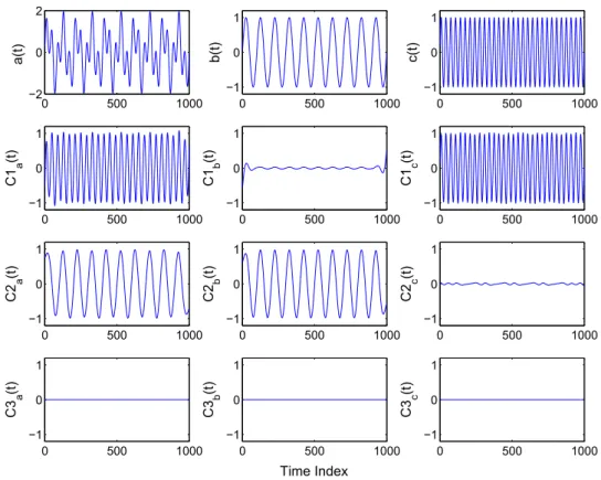
The multichannel processing capabilities of the MEMD can be demeonstrated with the following synthetic simulation, where the input to the MEMD is a 3-channel data
3
In theory, the filter bank property should produce IMFs that are partially well separated in frequency, thus reducing the effects of mode mixing.
source, containing the following sinusoidal oscillations:
a(t) = sin(2πf1t) + sin(2πf2t)
b(t) = sin(2πf1t)
c(t) = sin(2πf2t)
where f1= 100 Hz, f2 = 2f1 Hz, with sampling frequency of 1000 Hz.
Fig. 3.1 demonstrates the modal alignment properties of the MEMD algorithm. Where the conventional univariate EMD algorithm would result in IMFs for each channel that would vary in the number of IMFs as well as having IMFs that are not modally
0 500 1000 −2 0 2 a(t) 0 500 1000 −1 0 1 b(t) 0 500 1000 −1 0 1 c(t) 0 500 1000 −1 0 1 C1 a (t) 0 500 1000 −1 0 1 C2 a (t) 0 500 1000 −1 0 1 C3 a (t) 0 500 1000 −1 0 1 C1 b (t) 0 500 1000 −1 0 1 C2 b (t) 0 500 1000 −1 0 1 C3 b (t) 0 500 1000 −1 0 1 C1 c (t) 0 500 1000 −1 0 1 C2 c (t) 0 500 1000 −1 0 1 C3 c (t) Time Index
Figure 3.1: Simulation showing the MEMD decomposition of the three channel synthetic signal, a(t), b(t), c(t). It can be seen from the simulation the modal alignment of the corresponding IMFs. This would not be achieved using the single channel EMD, to process the three channels independently.