Fast Video Object Segmentation by Pixel-Wise Feature Comparison

Final Degree Research Thesis

Fast Video Object Segmentation by

Pixel-Wise Feature Comparison

A Real-Time approach to Video Object Segmentation

Degree in Industrial Engineering

&

Degree in Telecommunications Engineering

Author:

Rafel

_{Palliser Sans}

Supervisor:

Sanja

_Fidler

Home Tutor:

Xavier

_Gir´

_{o i Nieto}

Rafel Palliser Sans: Fast Video Object Segmentation by Pixel-Wise Feature Comparison. A Real-Time approach to Video Object Segmentation©, May 2019.

A Final Degree Research Thesis submitted to the Escola T`ecnica Superior d’Enginyeria In-dustrial de Barcelona (ETSEIB), Escola T`ecnica Superior d’Enginyeria de Telecomunicaci´o de Barcelona (ETSETB) and Centre de Formaci´o Interdisciplin`aria Superior (CFIS) of the Universitat Polit`ecnica de Catalunya (UPC) in partial fulfillment of the requirements for the

Doble Titulaci´o en grau d’Enginyeria Industrial i grau d’Enginyeria en Teleco-municacions, menci´o Telem`atica.

Thesis produced at the Vector Institute, University of Toronto, under the supervision of Prof. Sanja Fidler.

Supervisor:

Sanja Fidler

Home Tutor:

Xavier Gir´o i Nieto

Location:

If we want machines to think, we need to teach them to see.

— Fei-Fei Li

Abstract

Fast Video Object Segmentation by Pixel-Wise Feature Comparison is a

Real-Time approach to Video Object Segmentation, which tackles the task

of segmenting a video sequence with multiple objects with pixel resolution:

in every frame, each pixel must belong to an object. Solving Video

Ob-ject Segmentation would help a machine recognizing real-world scenes by

detecting and tracking objects. However, it can also be used as a tool to

build better and larger datasets easily, tagging all this ridiculous amount

of videos that are uploaded to the internet every hour.

The method that we present in this thesis is trained on the well-known

DAVIS dataset and evaluated on its own benchmark, taking into account

not only its accuracy but also its speed, aiming to be used in Real-Time

ap-plications. The final version of Fast Video Object Segmentation by

Pixel-Wise Feature Comparison (whose code is published at github.com/rafelps)

achieves a

G

Mean score of 71.1% on the DAVIS 2017 validation set while

running at 18 FPS, state-of-the-art results in both the accuracy and the

processing speed.

This thesis contains a concise introduction to Deep Learning and

Com-puter Vision as well as important Video Object Segmentation previous

work, and a full explanation of our approach to the task presenting

ab-lation studies on our different versions and modules, and a comparison

between our method and DAVIS benchmark’s best solutions.

KeyWords: Artificial Intelligence · Machine Learning· Deep Learning· Convolutional Neural Networks · Computer Vision · Video Object Segmentation · DAVIS dataset ·

ResNet · Feature Extraction · Pixel Embeddings· Pixel-Wise ·Real-Time ·PyTorch. 5

Acknowledgments

First of all, I would like to show my greatest gratitude to my supervisor

Prof. Sanja Fidler, for accepting me in her research group and guiding me

in my investigation project presented in this thesis.

I would also like to thank all Sanja’s group, and specially Xiaohui Zeng

for helping and giving me valuable advice. It has been a pleasure to be

part of that team, which is wondrous both personally and professionally.

I also need to thank the Vector Institute for its marvelous staff, its

lively workspace, and its research community. Thank you for letting me

use your offices, your computing resources and for all the high-quality talks

and activities you organized. I could not imagine a better place to work

on my project.

I would also like to thank the CFIS, Prof. Miguel ´

Angel Barja, Prof.

Eduardo Alarc´

on and Prof. Toni Pascual for the opportunities given to

me. Being able to produce my final degree research thesis in such an

outstanding place as Vector Institute is, and being supervised by one of

the most leading AI researchers worldwide, would not have been possible

without your work. Thanks also to Prof. Xavier Gir´

o for being my home

tutor, and to CFIS’ private sponsors for the grants given to the CFIS

international mobility program students.

I also wish to thank Eric Guisado, Ariadna Matabosch, Didac Sur´ıs

and Jordi Fortuny for helping me when things were not going as expected

and for celebrating together when good results arrived. Outside the office,

they were my family abroad, thanks for sharing many good moments.

Finally, I would like to thank my parents Rafel and Brigit, Miquel, and

F`

atima for encouraging me pursuing this opportunity and sending me the

warmth of my home, Menorca, in the distance.

Contents

1 Introduction 15

1.1 Motivation . . . 15

1.2 Objectives . . . 15

2 Artificial Intelligence, Deep Learning and Computer Vision 17 2.1 Artificial Intelligence . . . 17

2.2 Deep Learning . . . 18

2.2.1 Neural Networks . . . 18

2.2.2 Training Neural Networks . . . 18

2.3 Computer Vision . . . 20

2.3.1 Convolutional Neural Networks . . . 21

3 Video Object Segmentation 27 3.1 Video Object Segmentation: The task . . . 27

3.2 Video Object Segmentation datasets . . . 28

3.2.1 The DAVIS dataset and benchmark . . . 28

3.3 Previous work on Video Object Segmentation . . . 30

4 Fast Video Object Segmentation by Pixel-Wise Feature Comparison 33 4.1 The idea . . . 33

4.2 The Implementation . . . 34

4.2.1 Definitions . . . 34

4.2.2 Model Overview . . . 34

4.2.3 Individual Components’ Description . . . 35

4.2.4 Training Schedule . . . 39

5 Experiments and Results 41 5.1 Experiments on the model’s components . . . 41

5.2 Ablation Study on the model’s components . . . 44

5.3 Comparison of the state-of-the-art VOS methods . . . 45

6 Conclusions 47

Bibliography 49

Appendix A The Neural Network Zoo 53

Appendix B PiWiVOS’ per-object accuracy on DAVIS 2017 validation set 55 Appendix C PiWiVOS’ per-object accuracy on DAVIS 2017 test-dev set 57

Appendix D PiWiVOS’ visual results 59

List of Figures

2.1 Simple Neural Networks . . . 18

2.2 Rectified Linear Unit (ReLU) . . . 19

2.3 Sigmoid function . . . 19

2.4 Accuracy curve when training MNIST using different optimizers . . . 20

2.5 A convolutional layer with a single 3x3 filter . . . 22

2.6 A 2x2 Max Pooling layer . . . 22

2.7 A Fully Connected layer with 3 output cells . . . 23

2.8 ILSVRC. Evolution of top-5 error and architecture depth . . . 23

2.9 VGG’s architecture . . . 24

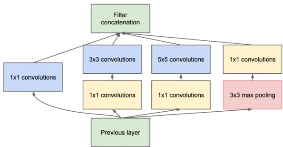
2.10 GoogLeNet’s inception module . . . 24

2.11 ResNet’s residual block . . . 25

2.12 Comparison of the most known architectures . . . 25

3.1 One-shot VOS with two objects to segment . . . 28

3.2 Comparison between DAVIS 2016 and DAVIS 2017 . . . 29

3.3 Visual representation of Intersection over Union . . . 29

3.4 Optical Flow . . . 31

3.5 ROI localization . . . 31

4.1 PiWiVOS’ Overview . . . 34

4.2 A single branch of the PiWiVOS’ pipeline . . . 35

4.3 ResNet versions and their layers . . . 36

5.1 Study of methods’ accuracy and speed on DAVIS 2017 validation set . . . 46

A.1 The Neural Network Zoo . . . 54

D.1 Qualitative results on the cow sequence . . . 59

D.2 Qualitative results on the horsejump-high sequence . . . 60

D.3 Qualitative results on the gold-fish sequence . . . 60

List of Tables

5.1 J mean,Fmean,Gmean and FPS for different ResNet versions and configurations

on DAVIS 2017 validation set . . . 41

5.2 J mean for different values ofλ0 on DAVIS 2017 validation set . . . 42

5.3 J mean for different values ofλt−1 on DAVIS 2017 validation set . . . 42

5.4 J Mean for different values ofK0 on DAVIS 2017 validation set . . . 42

5.5 J Mean for different values ofKt−1 on DAVIS 2017 validation set . . . 42

5.6 J mean and FPS for different branch merging options for output predictions on DAVIS 2017 validation set . . . 43

5.7 J mean for different branch merging options for loss function on DAVIS 2017 validation set . . . 44

5.8 J mean for the different options for loss function on DAVIS 2017 validation set . 44 5.9 Ablation Study on the model’s components . . . 44

5.10 J mean,F mean,Gmean and FPS comparison between the state-of-the-art VOS methods on DAVIS 2017 validation set . . . 45

5.11 J mean,F mean,Gmean and FPS comparison between the state-of-the-art VOS methods on DAVIS 2017 test-dev set . . . 46

B.1 PiWiVOS’ per-object accuracy on DAVIS 2017 validation set . . . 55

C.1 PiWiVOS’ per-object accuracy on DAVIS 2017 test-dev set . . . 58

Glossary

AI:

Artificial Intelligence

BCE:

Binary Cross-Entropy Loss

CNN:

Convolutional Neural Network

CV:

Computer Vision

DL:

Deel Learning

DNN:

Deep Neural Network

ML:

Machine Learning

NN:

Neural Network

RGB:

Red, Green and Blue. Used to refer to color images

RNN:

Recursive Neural Network

VOS:

Video Object Segmentation

1.

Introduction

1.1

Motivation

Artificial Intelligence is one of the most important technologies today. A proof of it can be seen, for example, in the automobile industry, where a few years ago electronics were the most significant innovations while nowadays everybody is talking about autonomous driving and other AI driving assistance. Moreover, some years ago, doctors struggled to diagnose some diseases; today machines help them improving their exactness in the diagnosis by recognizing tumors or analyzing electroencephalograms.

Artificial Intelligence is growing by leaps and bounds, and it is inevitable that we share our lives with AI machines in the next years. For this reason, it is an enormous motivation for me to carry on my final degree research thesis in this field.

Furthermore, as an engineer, I like to work on projects with clear applications in the real world, and Video Object Segmentation is an obvious example to it. Firstly, it processes videos which contain the temporal factor that image processing lacks. Then, it detects all types of objects what has many immediate applications like collision avoidance or helping robots interacting with real environments. Finally, it is a segmentation problem, which means that the detections are made in the highest resolution possible, pixel-wise.

1.2

Objectives

The first goal of this final degree research thesis is to understand how AI works without any prior knowledge of the technology. It is impossible to achieve good results without comprehending the fundaments and basics of its operation.

On the same direction, it is also crucial to get in touch with the previous work done in the specific task of Video Object Segmentation. Understanding the differences between the released methods, the reason of their architectures, how and why they work, and which are their weaknesses is a good starting point to begin designing our solution.

In terms of our model, there are several objectives that we want to accomplish. The most important one is that our method has to be fast. Fast enough to be used in Real-Time applications. As a consequence, an implicit objective is that our model is simple. On the other side, another essential aim is that it tackles the problem of multi-object segmentation in an intention to face real-world environments.

Last but not least, our designed architecture and method has to be implemented to validate its accuracy, speed, and effectiveness, what involves learning a new programming language or a Machine Learning framework to produce an efficient and clean implementation.

2.

Artificial Intelligence, Deep

Learning and Computer Vision

This chapter contains a brief introduction to Artificial Intelligence, and more specifically to the Deep Learning and Computer Vision technologies, jointly with a presentation of the most basic Neural Networks, and the main procedure to train them. In short, this chapter includes all the relevant prior knowledge needed for the research project presented in this thesis. It is the entrance door to the AI world.

2.1

Artificial Intelligence

Artificial Intelligence (AI) is used in many fields today such as data prediction, image classification, object detection or face recognition. It is an already immense but still growing world, and thus, one can find many definitions of it. Even so, the following one may contain all the necessary ingredients to describe it:

“Artificial intelligence is defined as the branch of science and technology that is concerned with the study of software and hardware to provide machines the ability to learn insights from data and the environment, and the ability to adapt to changing situations with high precision, accuracy and speed.”

— Amit Ray, Compassionate Artificial Superintelligence AI 5.0 So one could wonder: how can machines be provided the ability to learn? As Prof. Geoffrey Hinton once said, “the only way to get artificial intelligence to work is to do the computation in a way similar to the human brain”. The human brain is what gives us intelligence, what makes the human race different among all the other species. Although we still do not know exactly how our brain works, we know that it has a neural structure, so the AI aspiration is to replicate this structure into machines.

However, not only the architecture is replicated but also the way that humans learn. No child knows how to ride a bike from the first day he tries. In fact, it happens just the opposite, he slowly learns how to do it by practicing. The AI learning methodology is based on a repetitive approach, where the model gradually acquires knowledge by iterating.

18 CHAPTER 2. AI, DEEP LEARNING AND COMPUTER VISION

2.2

Deep Learning

2.2.1 Neural Networks

A Neural Network (NN) is, as its name says, a group of connected neurons. Biologically, a neuron has multiple stimuli (inputs) and generates a specific output signal depending on their combination. By simulating the human brain, in the AI world, a neuron is a node that performs the following linear function between its inputsx, and its output signaly:

y=W>x+b (2.1)

where W and bare the neuron’s weights and bias respectively, two own parameters. When we start grouping neurons such that the outputs of one layer are used as inputs for the succeeding one, we talk about a network. Every network has at least an input layer and an output one. However, any number of layers can be added between them. These are called hidden layers, and a NN with more than one of them is called Deep Neural Network (DNN). In the Figure 2.1a we can see the simplest network possible: a single output neuron with two inputs. On the other side, in Figure 2.1b, we can see an example of a DNN. Other configurations can be seen in the Network Zoo, in Appendix A.

(a) A neuron with two input cells. (b) A DNN with 3 input cells, 2 hidden layers with 4 neurons each and 2 output cells.

Figure 2.1: Simple Neural Networks. Input cells shown in yellow, hidden layers in green and output cells in orange.

2.2.2 Training Neural Networks

Training a NN means to reach a condition where the network has understood the data, and thus, it is able to make accurate predictions on it. There are many different network architectures, and data types, still, there are some generic steps that are used in most of the training schedules. In the first place, our data may need a preprocessing step depending on the dataset and chosen network, as many of them require normalized data. Furthermore, some architectures only accept input images with specific dimensions, so these may have to be resized or cropped. It is crucial that the data matches the network’s requirements.

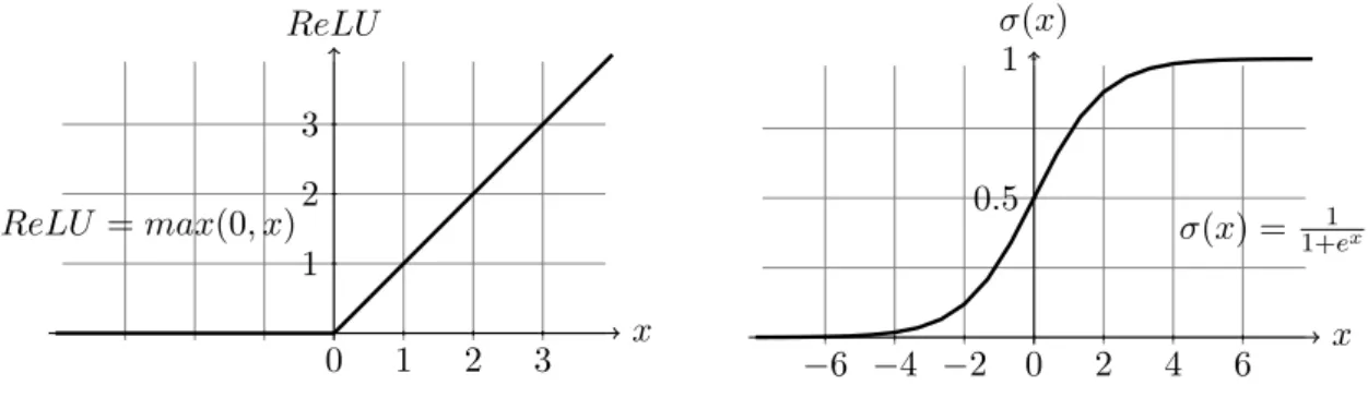
2.2. DEEP LEARNING 19 Once the data is in the correct format, it is time to forward-pass a data point into the network. As each neuron has a linear function (see Equation 2.1), we need to introduce some non-linearities. Otherwise, the composition of various linear functions would become a single linear function, and we would not take advantage of the hidden layers we introduced. These non-linear functions are called activation functions and are placed at the output of almost each neuron. ReLU (Figure 2.2) and Sigmoid (Figure 2.3) are the most used ones. While the former converts all negative outputs to zero, the later smoothly transforms the outputs fromRto the range [0,1]: x ReLU 0 1 2 3 1 2 3 ReLU =max(0, x)

Figure 2.2: Rectified Linear Unit (ReLU).

x σ(x) −6 −4 −2 0 2 4 6 0.5 1 σ(x) = ₁₊1_ex

Figure 2.3: Sigmoid function.

When the data point has forward-passed all the neurons and activation functions and arrives at the output of the last cell, a normalizing function may be used instead of an activation one. For example, in case that we have two outputs that should be probabilities, we would use a SoftMax function to normalize the outputs and force them sum to one. For a vector z of dimensionK, the normalized vector produced by SoftMax function σ(z) is:

σ :RK→ [0,1]K σ(z)j = ezj K−1 X k=0 ezk for all j∈ {0,1, . . . , K−1} (2.2)

After this function, our data point has been forward-passed through the whole network. To train our model, however, we need to give it some feedback on how accurate the predictions were. This accuracy is calculated in the loss or cost functions. In unsupervised methods, the loss functions compare different predictions between them, while when training in a supervised way, the predictions are compared to the ground truth. Some of the most used cost functions in supervised methods are L2 distance and Cross-Entropy Loss. The former is used in regression problems, where the target is continuous (see Equation 2.3 whereyˆis the prediction andy is the ground truth). On the other hand, Binary Cross-Entropy Loss is utilized in classification problems where the target is discrete (see Equation 2.4, where y denotes the ground truth, and

p is the probability for the predicted value of belonging to class 1).

L_L2(y,yˆ) = v u u t K−1 X k=0 (yk−yˆk)2 y= (y0, y1, . . . , yK−1), yˆ= (ˆy0,yˆ1, . . . ,yˆK−1) (2.3)

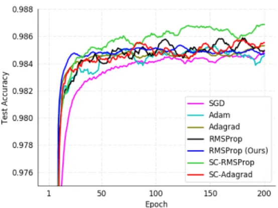
20 CHAPTER 2. AI, DEEP LEARNING AND COMPUTER VISION Once we have calculated the cost or error, we need to update the parameters (weights) of the neurons, so they adapt to the specific problem or data we are trying to learn. There are many optimizing algorithms such as Stochastic Gradient Descent (SGD), SGD Momentum, Adam, ... All of them are first-order algorithms, which means that they need the first order derivative of what we are minimizing (the cost) by respect to the parameters we want to optimize (the weights). There are higher-order algorithms, but they are not that popular.

The Backpropagation algorithm gives us these first order derivatives by differentiating the loss by respect to each weight by applying the chain rule inversely, backward. Note that this algorithm needs all the forward pass functions (the neuron’s forward function, activation functions, normalizing functions and the cost function itself) to be differentiable. It has to be remarked that one of the most used activation functions, ReLU, is not differentiable at 0. However, an approximation of its first derivative is employed, so there is no trouble in using it.

Figure 2.4: Accuracy curve when training MNIST using different optimizers.

These are the essential steps to train a net-work and have to be performed iteratively with all the data points used in training. In addition to this, there are a couple of other important concepts. On the one hand, if we use more than one data point in each forward-backward pass, we call it a batch. A larger batch size gives the optimizer more stability but needs more memory. On the other hand, when the whole training data has been passed through the network, we call it an epoch. It usually takes several epochs to train a network from scratch, although it is problem-dependent.

2.3

Computer Vision

Many different problems are being solved using Deep Learning today. Thus, one can find numerous different network structures, each of them optimized to be used for a specific task, or with a particular data type.

Machine Learning techniques and simpler NN are used for Big Data Analysis, for example. Problems such as Natural Language Processing (NLP) that rely on sequences (a series of words, for example), use Recursive Neural Networks (RNN) because its architecture has some memory to take advantage of previous outputted words. Additionally, there are different methods to train NN’s. Reinforcement Learning (RL) techniques rely on a reward function that they try to maximize while Generative Adversarial Networks (GANs) are two-role structures where the generator learns how to produce new synthetic data, and the discriminator learns how to distinguish synthetic from real data. Once trained, the discriminator cannot differentiate synthetic instances and so the generator, who has understood the dataset, can be used to create new data points.

One could write an entire book talking about different Neural Network structures. Neverthe-less, this thesis is focused on Computer Vision and Convolutional Neural Networks.

Computer Vision (CV) is a field of AI that aims at giving machines a visual understanding of images and videos similar to how human vision works. Its main difference with other techniques and architectures remains in its data type. Images have a clear two-dimensional spatiality, in

2.3. COMPUTER VISION 21 contrast to other kinds of data such as text, audio or simple scalars. In addition to this, a single image contains much more information than other data. For example, we could think of a Big Data problem where each data point can have thousands of features. A single RGB image at low resolution (480p) has 3 channels×480×854 = 1229760 values, three orders of magnitude larger, which encourages the idea that different architectures are needed.

In fact, these specific architectures utilized in Computer Vision, are called Convolutional Neural Networks and are used in many different tasks:

• Image Classification: This is one of the simplest tasks. Each image in the dataset contains a single object, which belongs to a previously known set of categories. The intention is to predict the object class.

• Localization + Classification: In this task, in addition to predicting the object category, the network has to prognosticate the object position inside the image by printing a bounding box around it.

• Object detection: In this problem, each image can contain multiple objects, and the goal is to detect them by printing a bounding box around every object in the picture. It can include object classification (among a set of known classes) or be class agnostic.

• Semantic Segmentation: To semantically segment an image means to assign each of the pixels to one of the possible classes, with prior knowledge of the collection of appearing categories, which usually includes abackground class.

• Instance Segmentation: Adds the difficulty of distinguishing instances of the same class. When assigning a label to each pixel in an image that contains, for example, two people, pixels belonging to the first person should be classified as personA, while pixels belonging to the other should be labeled aspersonB.

All the above are image processing tasks, but can be easily extrapolated to video sequences, as a video is no more than a sequence of frames. Some examples could be classifying a video where a single object appears, semantically segmenting all the pixels in every frame of the video or detecting and tracking a target throughout the whole sequence.

2.3.1 Convolutional Neural Networks

Convolutional Neural Networks (CNN) are a type of NN’s specifically designed to process images as they use their spatiality to extract additional information, and have a reduced number of weights in comparison to standard Neural Networks. CNN architectures are composed of three types of layers: convolutional layers, which are the most important and give the name to the whole network, pooling layers, and fully connected layers.

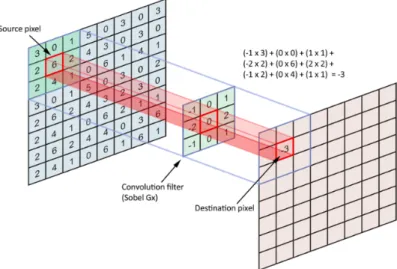
Convolutional layers are made of convolutional filters, and each of these filters also called kernels, has some learnable weights that are combined with the images’ values by dot products and sums. Figure 2.5 shows an example of a convolutional layer, with a 3x3 filter (9 learnable weights). The center of the kernel is placed above a pixel of the image, called source pixel, and it is weighted, jointly with its neighbors, by the kernel values. Finally, the results of all the products are added to produce one output value. The filter is then shifted to every other position to produce all the other outputs.

Furthermore, convolutional layers have some essential factors that slightly modify their behavior. On the one hand, we have the padding factor. To be able to operate in the edges, zero-padding or mirror-padding can be performed. On the other hand, the stride factor indicates

22 CHAPTER 2. AI, DEEP LEARNING AND COMPUTER VISION

Figure 2.5: A convolutional layer with a single 3x3 filter.

how many positions the kernel has to be shifted between operations. By default, stride one is used, so the center of the filter is placed to every input pixel, and spatial dimensions are conserved. However, larger strides can be employed to reduce output dimensionality as the center of the kernel is only placed to fewer input pixels.

Each of these convolutional filters produces a two-dimension output, which we call a feature map. However, in many computer vision tasks, more features drive to better predictions, so convolutional layers often have multiple filters, usually from 64 to 2048, each of them with its learnable parameters. For example, let’s think about a convolutional layer with 128 7x7 filters. If the layer’s input is an RGB image, each filter results in having 7×7×3 = 147 learnable weights, as color images have 3 channels. As we have 128 of them, we end up with approximately 19000 parameters and 128 feature maps, in front of the single output generated by a non-convolutional layer, with extremely more parameters (1230000 for a 480p resolution image). This is the potential of CNN’s and why they are perfect for image processing: they work with two dimensions (or more), incorporate context information in their operations, and save tons of computation resources.

In addition to convolutional layers, almost any CNN architecture incorporates some pooling layers. These are layers without learnable weights, so they are free in terms of computing memory, and its job is to reduce the spatial dimension of processed images. The idea is that extracted features at original dimension can give local information such as edges or colors but once the image is reduced using a pooling layer, resulting features have more global information, which is very useful for image classification, for example.

2.3. COMPUTER VISION 23 The most known pooling layers are Max Pooling and Average Pooling, and its behavior is very intuitive. Figure 2.6 shows a 4x4 input image passed through a 2x2 Max Pooling layer. Firstly, the image is split into regions of the layer’s dimension (2x2 in the example). Afterward, a reduction function is applied to each area generating an output value. In this case, the max operation is used while in Average Pooling, the output value would be calculated by the mean of the input region’s values.

Figure 2.7: A Fully Connected layer with 3 output cells.

Finally, there is a third kind of layer called fully connected layer (FC). These layers are usually used at the end of the networks, to sum up, and get the final predictions. For example, if we are classifying cats and dogs, the last layer would be a two cell FC layer, where each cell would give the probability of that image to contain one or the other animal. Each of these cells is connected to all of the outputs of the previous layer, so they are computationally costly because they have lots of learnable parameters. For example, classifying cats and dogs from an extracted feature space of 512 7x7 feature maps would imply 7×7×512 = 25088 weights for each cell, resulting in more than 50000 parameters for a single FC layer. One way of controlling it is by using some pooling layers before it, so the dimensions become smaller, and so does the number of learnable weights.

2.3.1.1 Most used CNN architectures

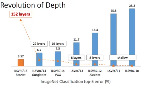
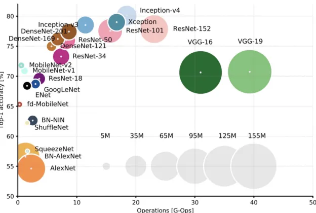
Although there are infinite combinations of layers, some of them work better than others in many tasks. The most used architectures, present in more than 85% of today networks are VGG [27] and ResNet [9]. Both of them were well-placed networks of the ImageNet Large Scale Visual Recognition Competition (ILSVRC) [26], an image classification challenge using the ImageNet dataset [5], which contains more than 14 millions annotated images belonging to more than 20000 different categories. The ILSVRC is, in fact, an excellent example to show the Computer Vision history.

24 CHAPTER 2. AI, DEEP LEARNING AND COMPUTER VISION On 2012, Alex Krizhevsky supervised by Geoffrey Hinton won the competition with AlexNet [15]. It was the first CNN that won the challenge and made a turning point as reduced the error rate by 10% to previous non-convolutional methods. The following year the first classified reduced the error by 5%, but the next revolutionary network was the 2014 runner-up, VGG [27], with more than three times the number of parameters, and more than twice the amount of layers, being able to reduce the top 5 error rate to 7.3%. They proved that it is better to have more layers with smaller kernels than vice versa, resulting in the same receptive field. Although it was the runner-up, it achieved the best top 1 error percentage (the benchmark is top 5 error).

Figure 2.9: VGG’s architecture.

Also on 2014, GoogLeNet [28] (playing tribute to Yan LeCun’s LeNet [16]), won the competition by increasing the number of layers to 22 but reducing the number of parameters significantly. They managed it by avoiding using FC layers. Moreover, they proposed some new ideas to train the network more efficiently, as introducing auxiliary outputs so the backward gradients could arrive to the first layers in better conditions.

2.3. COMPUTER VISION 25

Figure 2.11: ResNet’s residual block.

Finally, in 2015, the revolution of depth arrived. ResNet [9], the winner of that year’s competition, is a 152-layer residual network and achieved better accuracy than humans, which usually make a 5% error rate in the same task.

ResNet architecture is made of residual blocks. While a regular convolutional layer learns how to turn the input into the correct output, ResNet blocks only calculate which in-crement has to be added to the input identity to achieve the accurate output. These blocks have excellent properties such as better back-propagation and easiness in training the whole network, which is very important due to the immensity of itself and difficulty of gradients to not be vanished or exploded.

The project presented in this thesis uses a ResNet-50 backbone, as it has a perfect combination of limited use of computational resources, great extracted features and fast execution time.

Figure 2.12: Comparison of the number of parameters, computational cost, and accuracy of the most known architectures.

3.

Video Object Segmentation

This chapter includes the most relevant information about the task that the project presented in this thesis is treating: Video Object Segmentation. It includes a concise introduction to VOS, the existing VOS datasets, its most important benchmark to compare existing methods, and the most interesting approaches that have been proposed to solve the problem.

3.1

Video Object Segmentation: The task

Video Object Segmentation (VOS) tackles the problem of assigning a label to each pixel in each frame of a video shot, where a shot is defined as a sequence of frames without camera cuts. There are two main variants of the problem regarding the objects to be segmented: in the foreground-background task, a single object has to be separated from its background, while in the multi-object task, several objects have to be differentiated between them, even if belonging to the same category. This thesis is focused on multi-object VOS because it is a task closer to real-world environments, where different objects coexist and occlude each other. Furthermore, foreground-background can be seen as a specific case of multi-object where all the object masks are merged.

Moreover, VOS also has its variants in terms of supervision. Firstly, there is an interactive approach which aims to semi-automatically segment videos with the supervision of a human-in-the-loop, which can add control points to help the network know which objects has to segment. Secondly, we find the unsupervised or zero-shot approach, where the network has to decide which objects have to be segmented without any supervision. In this case, the network’s input are only the RGB images of the video sequence. Finally, there is the one-shot VOS, which is the most known and relevant approach today. It is called one-shot because the ground truth masks for the first frame are given, so we have one reference to identify which objects have to be segmented and how they look. This variant is also called weakly-supervised VOS or semi-supervised VOS. Even with these names, they are trained using supervised methods.

Furthermore, it is also important to know that Video Object Segmentation is a class agnostic task, which means that different objects that have to be segmented have to be given a unique label, but they do not have to be categorized into one class. However, some datasets have semantic annotations for further supervision.

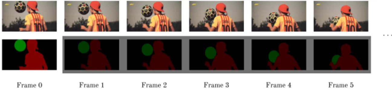
Figure 3.1 shows a multi-object class-agnostic one-shot VOS sequence, where the RGB frames for all the video and the ground truth masks for the first frame are given. Note that the masks are pixel-wise annotated, which means that each pixel has a label, which in this case is a color (the black color is reserved for the background). The objective is to extract the maximum information from the first frame’s masks to be able to predict where the objects are in the following frames, shadowed in grey. The fact that the green object is a soccer ball it is not important. However, it is crucial that all the pixels belonging to the soccer ball have the same tag in all the predicted masks.

28 CHAPTER 3. VIDEO OBJECT SEGMENTATION

Figure 3.1: One-shot VOS with two objects to segment from the background: Video frames and first frame ground truth masks are given. Shadowed, the goal, which is to predict all the other masks.

3.2

Video Object Segmentation datasets

Video Object Segmentation is a relatively new task, and therefore there are few datasets. Annotating segmentation masks for videos is a tedious and tough work, which also makes it difficult to have big datasets like ImageNet [5], CIFAR10 [14] or MNIST [17], that have image classification annotations.

SegTrack v2 [18] was in 2013 one of the first VOS datasets that appeared. It is formed by only 14 video sequences where 8 of them have a single object, 6 sequences contain 2 objects, and the penguin video exceptionally includes 6 instances. The sequences have an average of 70 frames although some of them have just 20, and others have more than 250. It is a tiny and varied dataset, which makes it challenging to train on it.

Later in 2016, DAVIS [23] dataset was presented, accompanied by an official benchmark. On 2017, a new multi-object version was released, jointly with a VOS challenge that already has 3 editions: 2017, 2018 and 2019. All these releases have made DAVIS the state-of-the-art dataset and benchmark for VOS, as different methods can be easily compared.

As DAVIS is not an enormous dataset, synthetic data or other non-VOS datasets are often used to train VOS methods more favorably before they are fine-tuned on the definitive data. YouTube-Objects [13], for example, has 720000 weakly annotated frames in terms of bounding boxes instead of segmentation masks, for the 10 categories of Pascal VOC Challenge [7]. Furthermore, Pascal VOC 2012 [6] extends its former challenge set of classes from 10 to 20 and provides object segmentation masks for almost 7000 static images. Finally, COCO [20] provides instance level segmentations for more than 90 object classes with an average of 10000 static images per class.

Recently, YouTube-VOS [33] has been released together with its own benchmark. It is almost 50 times larger than DAVIS in terms of frames and object variety, so it will become as known and as important as DAVIS sooner or later.

3.2.1 The DAVIS dataset and benchmark

DAVIS is the state-of-the-art benchmarking dataset for Video Object Segmentation. Its first version, DAVIS 2016 [23], contains 30 training videos and 20 validation sequences. The segmen-tations provided are foreground-background style, which means having a single mask per frame, even if there is more than one object.

3.2. VIDEO OBJECT SEGMENTATION DATASETS 29

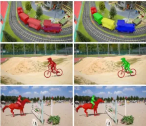
Figure 3.2: Comparison between DAVIS 2016 and DAVIS 2017 datasets. The former (left) has a single mask per group of objects as the latter (right) has a mask for each object to segment.

The following year, DAVIS 2017 [24] was released. It extends DAVIS 2016 training set to 60 videos, and its validation set to 30. Fur-thermore, the annotations are changed to be used in a multi-object instance segmentation environment. The same year DAVIS Chal-lenge [3, 24] was presented with two new sets of videos: test-dev set, with 30 new sequences and another 30 videos exclusively used in the challenge.

In DAVIS 2017 there are approximately 10500 annotated frames, leading to an average of 70 frames per sequence, and a mean of 2.5 objects per video. Although the dataset is not immense, their videos contain a wide variety of objects, huge pose variations, scale changes and occlusions and reappearances between the instances. These characteristics make the dataset incredibly challenging, and the proof of it is that the best method today has an accuracy lower than 70% on it while having more than 80% precision in other datasets.

All the training phases in this thesis use the original DAVIS 2017 training set, while evaluation is made under both the validation and test-dev sets.

In addition to all the annotated videos, DAVIS provides a benchmark [23] based on two metrics. On the one hand, the meanJ accard distance (J mean) also called mean Intersection over Union (mIoU), and on the other hand, theF-score(F) over the object boundaries.

For each frame, the J mean is calculated by averaging the individualJ accard distances for all the present objects. For each object, the IoU is the ratio between the intersection area and the area of union of the ground truth and the predicted masks. Alternatively, for each object,

J =IoU = T P

T P +F P +F N (3.1)

where T P (True Positives) is the number of pixels that were predicted as part of the object, and they really belonged to it; F P (False Positives) is the number of pixels that

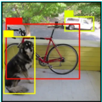
Figure 3.3: Visual representation of Intersection over Union where the green square acts as the ground truth mask, the red one as the prediction, and the areas of interest are filled in blue.

were predicted but did not belong to the object; andF N (False Negatives) is the number of object pixels that were not predicted.

30 CHAPTER 3. VIDEO OBJECT SEGMENTATION The F-score, by its side, is a ratio between Precision (P r) and Recall (Rc). The former calculates how many of the predicted pixels are relevant while the latter measures how many of the relevant items have been predicted:

F = 2· P r·Rc P r+Rc (3.2a) P r= T P T P +F P (3.2b) Rc= T P T P +F N (3.2c)

In the DAVIS benchmark, the F-score is measured on the masks’ boundaries, which means that in this case,T P is the number of pixels that were predicted as belonging to the boundary of the object mask, and they indeed were. The equivalent is applied toF P and F N definitions.

A boundary is defined as the pixel were an object ends, or another one starts. Predicting the exact border pixel in a 480p image is incredibly difficult. For this reason, the DAVIS boundary

F-score has a certain margin (around 8 pixels), and any predicted edge pixel that is located inside this margin is computed as correct.

Finally, DAVIS benchmark defines an additional metric to summarize the accuracy of a method, theG mean. It is calculated as the mean between the J mean and theF-score:

G= J +F

2 (3.3)

The global benchmark for a specific method on a video set (training, validation or test-dev) is obtained as the mean of all the sequences in it, while the values for each sequence are obtained averaging the scores of each of the individual frames, which at the same time are calculated averaging the scores for every object in them.

3.3

Previous work on Video Object Segmentation

Since now, there have been many different approaches to Video Object Segmentation. Although all of them are different, there are two main basic ideas: Object Detection and Mask Propagation.

Object Detection methods mostly rely on the first frame, learning the appearance of the object to be segmented from the given masks and trying to detect it in the following frames. They process video sequences as individual images, without using temporal consistency, so they usually suffer from appearance changes in non-solid objects (e.g. people or animals), scale and pose variations.

Caelleset al. in OSVOS [2] online fine-tune their model for each sequence, in order to learn the exact appearance of the object to be separated from its background. Then, they process the other frames one by one, without using temporal information. In OSVOS-S [22], they incorporate a semantic supervision to their previous method improving their results. As they only use the object appearance of the first frame, they need to train for several iterations until the network learns the specific task of segmenting that particular object. This online fine-tuning step on test time impede both methods to be time efficient.

3.3. PREVIOUS WORK ON VIDEO OBJECT SEGMENTATION 31 By its part, Hu et al. in VideoMatch [11] also use the first frame exclusively but in a different manner. They extract features from it for both the objects and the background to then compare them to the extracted features of each other frame. Additionally, Voigtlaenderet al. in OnAVOS [30] implement the ability to adapt and update the reference appearance of the objects in the first frame to cope with aspect variations while processing the whole sequence. Both methods add online fine-tuning to achieve better results, having the same time efficiency problem.

On the other hand, we can find the Mask Propagation based methods. These models often use optical flow to warp predicted masks of previous frames according to the motion of the video. They rely on temporal consistency, and thus, recursive networks are often used.

Hu et al. in MaskRNN [10] use FlowNet 2.0 [12] to extract optical flow between adjacent frames and use it to propagate the first frame ground truth masks through all the video, while Baoet al. use a similar idea and incorporate an MRF postprocessing step in CINM [1].

Figure 3.4: Optical Flow generated from FlowNet 2.0 between adjacent frames. Red areas show where movement is while static areas are painted in blue.

Their heavy reliance on the previous frame predicted masks make them vulnerable to occlusions, as when an object disappears they do not have any mechanism to retrieve them. Furthermore, they rely on previous predictions instead of ground truth, which has the risk of degenerating if predictions are not good enough.

As both Image Detection and Mask Propagation have their benefits, it is easy to find some models that combine both of them in order to avoid the problems they have individually.

Oh et al. in RGMP [32], for example, use a siamese network where one of its branches is dedicated to a reference frame (the first one), and the other one to the last processed frame. Combining two references gives them some robustness against pose variation and occlusions. SiamMask [31] also uses a siamese network to take advantage of the previously predicted masks. Any of them need online fine-tuning which converts them into fast and time efficient methods.

Figure 3.5: Region of Interest localization output with 3 detected objects.

Furthermore, FAVOS [4], DyeNet [19], and PRe-MVOS [21] use a Region Of Interest localization network (such as Mask-RCNN [8]) to retrieve new objects that appear in farther frames and compare them to previ-ously stored templates of the objects of interest. This re-identification mechanism helps them when objects are occluded, or significant appearance variations happen. In addition to this, DyeNet and PReMVOS also use optical flow to warp the masks of previously processed frames in accordance with the video movement.

32 CHAPTER 3. VIDEO OBJECT SEGMENTATION Mixing object detection, re-identification, and mask propagation techniques lead them to state-of-the-art results. However, these are time consumptive methodologies, and combining them with online fine-tuning or postprocessing steps make these models dilatory.

Finally, RVOS [29], recently presented by Venturaet al., is an extremely rapid spatiotemporal RNN architecture where the spatial branch predicts all the objects for a specific time step and the temporal section is which contains all the previous time steps memory. Apart from being a solution to the one-shot problem, it is one of the first approaches to face the zero-shot unsupervised task.

4.

Fast Video Object Segmentation

by Pixel-Wise Feature Comparison

This chapter is meant to be the principal episode of this thesis because it contains the presented solution to Video Object Segmentation. After a brief explanation of the idea behind it, this chapter also includes an overview of the proposed model and a complete description of each of its individual components. Finally, it also contains some information about the training schedule followed to lead the model to state-of-the-art results.

4.1

The idea

Nowadays, 3 hours of video are uploaded to YouTube every second. We would need more than 10000 humans working all day, every day to process, tag and classify this enormous amount of data, so it is evident that we need algorithms for machines to do this work. Furthermore, video has become more and more important due to growing technologies such as autonomous driving.

Many researching groups have detected this need for developing useful VOS methods. However, most of them end up with very complex networks and algorithms that often need tens or hundreds of seconds to process each photogram.

The goals of Fast VOS by Pixel-Wise Feature Comparison (PiWiVOS) are to be simple and fast enough to be used in Real-Time applications. Furthermore, in the same aim to be used in real-world environments, our method is directly addressed to the multi-object VOS problem. One can easily see that almost all the existing VOS models, presented in Section 3.3, start solving the foreground-background segmentation problem, to then move to the multi-object task by merging their results. Even those methods that are prepared and trained for multi-object segmentation directly, need a forward pass for each of them or an RNN to predict them one by one. All the previously presented approaches are object-wise methods.

In contrast, our model PiWiVOS is a pixel-wise approach, where with a single forward pass, pixel embeddings are extracted and compared with previously obtained features of two different references: the first frame (where ground truth masks are given) and the predictions of the previous time step. This simplistic approach leads our method to state-of-the-art results in both its accuracy and its processing speed.

34 CHAPTER 4. FAST VOS BY PIXEL-WISE FEATURE COMPARISON

4.2

The Implementation

4.2.1 Definitions

Let I = {I0_{, I}1_{, . . . , I}t_{, . . . , I}T−1_{} be the given sequence of T RGB images. Furthermore, let}

ˆ

yt∈ {0,1, . . . , n, . . . , N−1}H×W _{be the prediction for frame twhere H andW are the original}

height and width of the video, andndenotes the predicted object for each pixel among the N

possible objects, including background, which is represented as n= 0. Finally, let y0 be the given ground truth masks for the first frame.

4.2.2 Model Overview

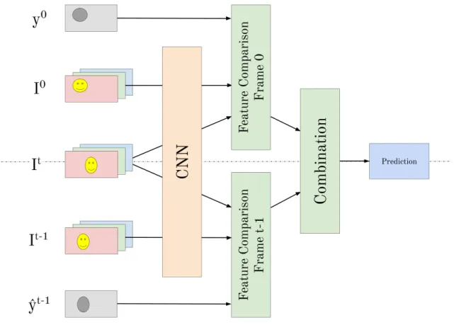
PiWiVOS has two parallel branches, each of them processing the current frame and comparing it to a particular reference frame. The first section uses the first frame,I0 (where ground truth masks are given y0) as guidance, while the second branch matches the processed frame to the previous one, It−1, using the earlier predicted masks ˆyt−1. Finally, the result of both branches are combined to produce the output predictions. Both branches are exactly the same and share the CNN weights.

Figure 4.1: PiWiVOS’ Overview.

The inputs of each branch are two RGB images, It, and Ireference, which is either I0 or

It−1. Each image is individually forward-passed through a feature extractor, generating a low-resolution feature volume. Both feature volumes are compared with the guidance of the reference masks (eithery0 or ˆyt−1), and a pixel-wise object score map is generated, where every pixel in the low-resolution dimensions has a score list of belonging to one object or the other.

4.2. THE IMPLEMENTATION 35

Figure 4.2: A single branch of the PiWiVOS’ pipeline.

This score volume is then used to generate three different outputs. Firstly, it is bilinearly upscaled to the dimensions of the input image, and combined with the other branch upscaled volume. The highest scored object (pixel-wise) is chosen to be the final prediction. Secondly, the low-resolution score volume is also combined with the other branch’s scores to output a low-scale prediction, which will be used in the subsequent time step as reference masks in the comparison module. Finally, when training, these scores are normalized into probabilities using the SoftMax function, combined with the other branch object probabilities, and lastly compared to the ground truth by the loss function.

Hereafter, each component of the method will be individually presented and described.

4.2.3 Individual Components’ Description

Data Preprocessing

DAVIS 2017 videos are given as sequences of individual RGB images with 8-bit codification for each of their 3 channels. They are provided on both Full-Resolution and 480p, although the benchmarks are calculated on the 480p predictions. In order to use these images with a CNN, a linear normalization is performed in each of their three channels, re-scaling their values from [0,255] to [0,1].

On the other side, the ground truth masks are given with a single-channel palette-mode image where each integer value represents an object: pixels with the value 0 belong to background, those with value 1 are classified as object1, and so on. The ground truth masks do not need any preprocessing.

The predictions must be exported with the same format than the ground truth masks to use the DAVIS’ automatic benchmarking tool.

36 CHAPTER 4. FAST VOS BY PIXEL-WISE FEATURE COMPARISON The Feature Extracting Network

The chosen architecture for feature extracting is ResNet-50, which is a 50-layer reduced version of the original ResNet, which has 152. As explained in Section 2.3.1, CNN’s tend to reduce the spatial dimensions while increasing the number of channels or feature maps. If we obviate the final fully connected layer, ResNet-50 outputs 2048 channels where the height and width have been reduced by a factor of 32 in respect to the input image. Although this is acceptable when performing image classification, in segmentation problems we require a dense output as each pixel has to be labeled.

PiWiVOS uses the first 4 layer blocks of ResNet-50 (see Figure 4.3), from conv1 to conv4 x. Furthermore, the stride of the convolutional layers in the last block (conv4 x) is reduced from 2 to 1 to have four times the number of outputted pixels. The resulting extracted volume consists of 1024 features with a reduction of 1/8 in both the height and the width in respect with the original input image. It is a perfect balance between the number of features, their receptive field, and the output dimensions for a segmentation task.

Figure 4.3: ResNet versions and their layers. Note that output size is relative to the input.

The Feature Comparison Module

The feature comparison module is the most essential part of the method because it is the one that enables the pixel-wise approach and permits to generate a multi-object prediction by only forward-passing each frame once.

Their inputs are the extracted feature volume for the current frame,ft∈_Rh×w×1024 _(where

h andw are the reduced height and width respectively), the feature volume for the reference framefref ∈Rh×w×1024, and the reduced reference masksyref ∈ {0,1, . . . , N−1}h×w. Note that the reference can either be the first frame or the previous one, whereyref would become ˆyt−1. For the rest of the explanation we will useyref as both the ground truth for frame I0 and the predicted masks for frameIt−1.

Once we have the inputs, for each pixel iin the reduced dimensions of the current frame t, we take its feature vector f_it∈R1024 and we compare it with the feature vector fjref of every

pixelj in the reference, generating a similarity score sref_i,j:

4.2. THE IMPLEMENTATION 37 similarity(f_it, f_jref) = f t i > ·f_jref kft ik · kfjrefk −λ·distance(i, j) λ∈[0,1] (4.1b) distance(i, j) = p (ix−jx)2+ (iy−jy)2 p (h−1)2_{+ (w−1)}2 (4.1c)

where λ is a parameter that penalizes the possible fact that two separate pixels have similar features, and xand y are the Cartesian coordinates for the pixel of interest inside the two-dimension reduced image.

After comparing pixel i with each of the pixels j in the reference frame, these similarity scores sref_i,j are converted to a single vector of object scoresoref_i :

oref_i = (oref_i,0, oref_i,1, . . . , oref_i,n, . . . , oref_i,N−1) (4.2)

where each of these entries contains the score of pixelito belong to objectnand is calculated as follows:

oref_i,n= avg   topK j|yref j =n (sref_i,j)   for all n∈ {0,1, . . . N −1} (4.3)

where the topK operator selects theK highest scoredsref_i,j. The value of the parameter K, which allows avoiding outliers, will be discussed in Section 5.1.

All these calculations are made for each pixel i∈ {0,1, . . . , h·w−1}. When put together, it results in an object scores volume of dimensions h×w×N.

Object Scores merging

After calculating the object scores with the frame I0 as a reference, o0_i, and those with the previous frame, ot_i−1, both of them are combined to produce three outputs.

To calculate the final prediction, each of these object score volumes is upscaled to the dimensions of the input images (note that the dimensions had been reduced inside the CNN) by bilinear interpolation. Afterward, for each pixel i, both object score vectors, o0_i andot_i−1, are combined by taking the maximum score object-wise, resulting inoi. The predicted object is

chosen by taking the index of the highest score in the array

oi= (oi,0, oi,1, . . . , oi,n, . . . , oi,N−1) (4.4a)

oi,n= max(o0i,n, ot

−1

i,n ) for all n∈ {0,1, . . . , N−1} (4.4b)

ˆ

yi= argmax n

(oi,0, oi,1, . . . , oi,n, . . . , oi,N−1) (4.4c)

The same process is followed to generate the low-scale prediction (without upscaling) that will be used in the succeeding time step.

38 CHAPTER 4. FAST VOS BY PIXEL-WISE FEATURE COMPARISON To produce the last output, however, it is crucial to take into consideration that it is not the same combining the scores to produce a prediction, than using them to calculate the loss. In this last case, the loss needs to be fed normalized probabilities in order to work correctly. For this reason, each object score vector is normalized by the SoftMax function (σ()) separately. Then, for each pixel iboth probability vectors are combined in the following weighted sum:

pi,n=wcomb·σ(o0_i)_n+ (1−wcomb)·σ(ot_i−1)_n for all n∈ {0,1, . . . , N−1} (4.5)

Weighted multi-class Cross-Entropy Loss

As seen in Section 2.2.2, Binary Cross-Entropy Loss is the most utilized cost function in classification problems where the target has two possible discrete values, either cats and dogs or 0 and 1. Its operation is simple: in this last example, for the case when the ground truth is 1, the predicted probability is “pushed” towards 1 proportionally to the logarithmic distance between the prediction and the target value, 1 (see Equation 2.4).

The multi-class scene does not differ that much from the binary problem. The main difference is that it does not have a single predicted value anymore, but a prediction for each of the objects or categories. As a consequence, the multi-class Cross-Entropy Loss forN objects, where the predicted probabilities are pn forn∈ {0,1, . . . , N−1}, and the correct object is n∗, looks like:

L_CE =−log(pn∗) (4.6)

Note that although it seems that the loss function is only working on pn∗, in addition to

pushing it to 1, it is implicitly pushing all the other probabilitiespn|n6=n∗ to 0 as they must add

to 1.

In our pixel-wise approach, the Cross-Entropy Loss is applied to all the pixels individually, to be then averaged for the whole frame, which has a potential problem.

Let’s imagine a scenario where all frames contain one single object apart from the background. If these frames have an average of 90% of background pixels, and only 10% of its pixels belong to the object, the network can eventually learn to predict everything as background, and stabilize with a quite small loss. This situation is prevalent in the DAVIS dataset sequences, where this behavior is not desired as all the objects are equally important.

A weighted version of the multi-class Cross-Entropy Loss is proposed to solve this problem: LCE =−wn∗log(p_n∗) (4.7a) wn= 1 |{y|y=n}| N−1 X k=0 1 |{y|y=k}| for all n∈ {0,1, . . . , N−1} (4.7b)

where |{y|y = n}| is the number of ground truth pixels labeled as object n in the whole frame.

4.2. THE IMPLEMENTATION 39 Thereby, in our model, the following equation is used to calculate the loss for each frame:

L= avg i (Li) = avg i (−wn∗ ilog(pi,n ∗ i)) (4.8)

where n∗_i is the correct object for each pixeli.

4.2.4 Training Schedule

This model is trained using ResNet-50 pre-trained weights on ImageNet directly downloaded from the torchvision model zoo [25]. From this starting point, it is then fine-tuned on the DAVIS 2017 training dataset using the Stochastic Gradient Descent Momentum optimizer, with hyperparametersλ= 5e−4 and β= 0.9.

The model is trained for 30 epochs during 12 hours on a single Nvidia Titan XP GPU, using a mini-batch size of 1 due to memory limitations (each batch contains the processed frame, its previous frame and the first frame of the sequence).

The implementation of PiWiVOS, coded in Python using the PyTorch library, has been published on https://github.com/rafelps/PiWiVOS.

5.

Experiments and Results

This chapter contains all the experiments and results that empirically substantiate each of the parameters’ value and component design. Furthermore, it also includes an ablation study on the performance of each component of the method, and a comparison of the accuracy and speed of the most relevant Video Object Segmentation approaches.

5.1

Experiments on the model’s components

In this section, we discuss the decision of selecting each of the chosen components and parameters. In each of the individual experiments, all the parameters that are not analyzed are kept constant. The Feature Extracting Network

It is well known that deeper networks usually have better results due to their larger capacity to adapt to new data. However, more layer implies more parameters and more computation resources, both time and memory. In addition to the number of layers, the stride factor in the conv4 x layer changes the outputted feature volumes. When the stride is 2, the dimensions of the input image are reduced by a factor of 16 in both the height and the width. However, when the stride is set to 1, the reducing factor becomes 8, so the output becomes 4 times larger, which makes the method slower as it has to process larger tensors. In the following experiment, we compare different versions of ResNet to choose the one that best fits our objectives.

ResNet version conv4 x stride J Mean F Mean G Mean FPS

ResNet-34 2 55.7 54.0 54.9 85

ResNet-50 2 56.6 54.7 55.7 56

ResNet-101 2 59.4 56.2 57.8 35

ResNet-34 1 64.3 70.7 67.5 26

ResNet-50 1 67.6 74.6 71.1 18

Table 5.1: J mean,F mean,G mean and FPS for different ResNet versions and configurations on DAVIS 2017 validation set.

There is a clear relationship between the output dimensions (higher outputs lead to more resolution in our predictions), the number of layers, the model accuracy, and its speed: more computation means better results but a slower method. However, the slowest solution, ResNet-50 (conv4 x stride 1), is already faster than almost every other published method, achieving state-of-the-art results. For this reason, it is the chosen backbone for PiWiVOS.

Nevertheless, our approach is fully compatible with all the presented versions of ResNet. Therefore, for other applications that do not need state-of-the-art accuracy, ResNet-34 (conv4 x stride 2) could also be an interesting choice as it is 1500 times faster than other methods with similar accuracy. We will call this approach PiWiVOS-Fast.

42 CHAPTER 5. EXPERIMENTS AND RESULTS The Feature Comparison Module

The first parameter to be analyzed in the feature comparison module is λ, which penalizes the possible fact that two separate pixels have similar features (see Equation 4.1b). It may be interesting to use differentλ’s for each branch, so the following values for λ0 _andλt−1 _{have been}

studied:

λ0 0 0.25 0.5 0.75 1 J Mean 64.0 67.4 67.6 67.0 66.1

Table 5.2: J mean for different values ofλ0 _{on DAVIS 2017 validation set.}

λt−1 _{0 0.25 0.5 0.75 1}

J Mean 63.4 66.8 67.6 67.6 67.3

Table 5.3: J mean for different values of λt−1 on DAVIS 2017 validation set.

It can easily be seen that in both branches the λpenalization improves the accuracy as the worst results happen when λ= 0. Furthermore, the model seems to work better withλ0_≤λt−1_,

which also makes sense. Video sequences contain continuous motion, and therefore objects in adjacent frames (t, t-1) have to be relatively close, or at least closer than when comparing the last frames with the first one, where it is possible that objects have different positions.

Following, there is an analysis of the parameterK, presented in Equation 4.3. Analogously as withλ, different values ofK may work on each branch. For this reason, parametersK0 and

Kt−1 are defined.

K0 1 2 3 5 10 all

J Mean 67.6 67.1 66.8 65.7 64.1 52.3

Table 5.4: J Mean for different values of K0 _{on DAVIS 2017 validation set.}

Kt−1 1 3 5 10 15 all J Mean 52.4 64.0 66.0 67.6 66.9 54.3

Table 5.5: J Mean for different values of Kt−1 on DAVIS 2017 validation set.

The results of this experiment are also logical. In the first branch, where the reference is the ground truth of the first frame, the calculated similarity scoress0_i,j are very reliable, so the best performance is achieved whenK is set to 1. In this case, the object score o0_i,n takes the information of one single pixel in the reference frame:

o0_i,n= avg  top1 j|y0 j=n (s0_i,j)  = avg max j|y0 j=n (s0_i,j) ! = max j|y0 j=n (s0_i,j) (5.1)

However, in the second branch, ground truth is not available and we work on previous predictions. In this case, a value of 10 works the best because when averaging scores between

5.1. EXPERIMENTS ON THE MODEL’S COMPONENTS 43 pixel iand 10 different pixelsj that belong to objectnon the reference frame It−1, the variance of the prediction is reduced.

ot_i,n−1 = avg   top10 j|yˆt_j−1=n (st_i,j−1)   (5.2)

Note that when K is set toall, the performance drops. In this case, the operator topK does not intervene, so the object scoreoref_i,n is calculated by averaging all the similarity scores between pixeli and every pixelj in the reference frame that belongs to objectn. This does not work because not all the pixels of an object have the same features.

oref_i,n= avg  topall j|yref j =n (sref_i,j)  = avg j|yref j =n (sref_i,j) (5.3)

In addition to all the results presented in Tables 5.2, 5.3, 5.4 and 5.5, many experiments were made with different combinations of values for K0, Kt−1, λ0 andλt−1. They seem to work quite independently, and the best performance is achieved with the following combination:

K0 = 1 Kt−1 = 10 λ0 = 0.5 λt−1 = 0.5

Object Scores merging

Several options have been studied to merge the two branches’ object score volumes:

• Option A:oi,n= max(o0i,n, ot

−1 i,n )

• Option B:oi,n=w·o0i,n+ (1−w)·o t−1 i,n

• Option C: oi,n=σ(oi,0, . . . oi,N−1)n where oi,n= max(o0i,n, o t−1 i,n)

• Option D:oi,n=w·σ(o0i,0, . . . , o0i,N−1)n+ (1−w)·σ(oti,−01, . . . , ot

−1 i,N−1)n

where σ() is the SoftMax function described in Equation 2.2, andw∈[0,1] is a weight.

Option A B w= 0.25 B w= 0.5 B w= 0.75 C D w= 0.25 D w= 0.5 D w= 0.75 J Mean 67.6 61.2 62.0 62.7 63.4 61.4 61.5 62.7 FPS 18 18 18 18 14 14 14 14

Table 5.6: J mean and FPS for different branch merging options for output predictions on DAVIS 2017 validation set.

It results that the best option is to use the max function instead of a weighted sum, and the raw scores better than normalized ones, which is an advantage for the time efficiency because calculating the SoftMax function pixel-wise carries a slowdown of 4 FPS.

However, when we have to merge the results to feed the loss function, they have to be normalized, so a different analysis is made for this particular case with options C and D.

44 CHAPTER 5. EXPERIMENTS AND RESULTS Option C D wcomb = 0 D wcomb = 0.25 D wcomb = 0.5 D wcomb = 0.75 D wcomb= 1 J Mean 66.7 66.5 66.7 66.9 67.5 67.6

Table 5.7: J mean for different branch merging options for loss function on DAVIS 2017 validation set.

In this case, the best option to feed the loss function is to directly give it the normalized vector of object scores from the first branch, where the reference is the first frame and we have the ground truth masks available. We can interpret that predictions coming from the first branch are more reliable and stable, so they lead to a better training. Note that this does not mean that the second branch is dispensable because their scores are still being used to calculate the final predictions, as will be seen in Section 5.2.

Weighted multi-class Cross-Entropy Loss

Finally, a simple study on the proposed Weighted multi-class Cross-Entropy Loss has been made: Cross-Entroy Loss Weighted Non-Weighted

J Mean 67,6 66,9

Table 5.8: J mean for the different options for loss function on DAVIS 2017 validation set.

It can be seen that the weighted loss gives the model a boost in performance, which is logical as it helps to give each object the same importance.

5.2

Ablation Study on the model’s components

In this section, an ablation study has been performed to confirm the effectiveness of each component of our method. Pre-trained experiments use the pre-trained weights of ResNet on Imagenet, without fine-tuning on DAVIS, while −K and −λ mean using the values 1 and 0 respectively instead of the optimal ones, and−branch means that this part of the model is not used. Configuration J Mean Pre-trained −branch 0 47.4 Pre-trained −brancht−1 52.4 Pre-trained −K −λ 47.4 Pre-trained −K 47.6 Pre-trained −λ 52.8 Pre-trained 59.3 Configuration J Mean PiWiVOS −branch 0 58.8 PiWiVOS −brancht−1 57.3 PiWiVOS −K −λ 54.3 PiWiVOS −K 54.5 PiWiVOS −λ 63.8 PiWiVOS 67.7

Table 5.9: Ablation Study on the model’s components.

It can be seen that each of the method’s components, including the training schedule, is crucial to reach state-of-the-art performance. The topK operator is the one that gives the most significant boost (+13.2%), while the distance penalizationλgives the least (+3.9%). In addition to this, the fine-tuning stage on DAVIS training set improves the method’s accuracy approximately 10%. Finally, note that although outputs of thet−1 branch are not used in the