Implementation of an interactive visualization tool for analyzing dynamic hierarchies

(1)

Institut f¨ur Visualisierungsinstitut Universit¨at Stuttgart Allmandring 19 D-70569 Stuttgart Master’s thesis Nr. 3340

Implementation of an Interactive

Visualization Tool for Analyzing

Dynamic Hierarchies

Christine Louka

Course of Study: Infotech

Examiner: Prof. Dr. Daniel Weiskopf

Supervisor: Dr. rer. nat. Michael Burch

Commenced: May 15, 2012

(2)

(3)

Abstract

Many real world examples can be found that deal with hierarchical data. Software sys-tems typically consist of packages, directories, subdirectories, files, classes, and functions. Phylogenetic trees structure biological species into a hierarchical organization. Visualiz-ing such static hierarchical data has been in focus of Information Visualization for many years. Visually encoding and understanding of evolving hierarchies still remains a chal-lenging task. Since hierarchies may grow huge and may evolve over a long time producing many time steps, we make use of a side-by-side and aligned representation of Indented Pixel Tree Plots. To achieve a mental map preserving overview-based diagram we show the dynamics of a hierarchy by a static representation and illustrate the changes between subsequent hierarchies by special links. Interactive features make the data manipulable and navigable in all dimensions.

(4)

(5)

Acknowledgement

First and foremost I would like to thank God for his blessings, support and the strength he gave me.

It gives me great pleasure in acknowledging the support, help and guidance of Dr. rer. nat. Michael Burch. Thank you for your fast e-mail replies even when you were on business trips or holidays.

I also want to thank my friends in Stuttgart whom I cannot find words to express my gratitude to, Mirna Aiman, Michael Guirguis, Mariam Hassib, Ghada dessouky, Youssef Ghaly, Pierre Ibrahim, Mina Metias, Ahmed Halawa and Amr yassin. It was a two year journey and they have always been there supporting and helping me all the way, I cannot thank them enough.

This thesis would not have been possible without my parents’ encouragement and insistence on travelling and doing my masters abroad, so a big thanks to my mother and my father as well as to my twin sister Sandra Louka who was there whenever I needed her the most with her love and patience.

And last but not least, I would like to thank my friends and family in Egypt for their prayers and support from long distance. They always cared on asking me how I am doing and always encouraged me.

Each of you can share in this accomplishment, for without your support it would not have been possible.

(6)

(7)

List of Figures

1.1 Node-link diagram of a hierarchy in a top-down layout . . . 1

1.2 The changes of a hierarchical organization . . . 2

2.1 Visual metaphors for hierarchical data . . . 5

2.2 Node-link diagram . . . 7

2.3 Di↵erent Treemap layouts . . . 8

2.4 Nested Treemap . . . 9 2.5 Cushion Treemap . . . 10 2.6 Pebble Treemap . . . 10 2.7 Voronoi Treemap . . . 11 2.8 Cartesian layout . . . 12 2.9 Sunburst layout . . . 13 2.10 Information slices . . . 14

2.11 Angular detail technique . . . 15

2.12 Operations implemented for interactivity on hierarchical structures . . . 16

2.13 Windows Explorer . . . 17

2.14 Indented pixel tree plot . . . 18

2.15 Elastic hierarchy . . . 20

2.16 IPTPs compared . . . 22

3.1 IPTP representing the ’NCBI taxonomy’ highlighting a subregion . . . . 24

3.2 IPTP representing the ’NCBI taxonomy’ illustrating the deepest leaf nodes 25 3.3 IPTPs of the ’dblp.newick.100’ file . . . 26

3.4 Hierarchy Legend . . . 26

3.5 IPTPs of the ’dblp.newick.100’ file after comparison . . . 27

3.6 IPTPs of the ’dblp.newick.100’ file after applying filters . . . 28

3.7 IPTPs of the ’dblp.newick.100’ file after a node search . . . 29

3.8 IPTPs of the ’dblp.newick.100’ file after applying the time filter . . . 29

3.9 IPTPs of the ’dblp.newick.100’ file after multiple filter application . . . . 30

3.10 Information on specific IPTPs . . . 31

4.1 Process overview diagram . . . 33

4.2 Class diagram (1) . . . 35

4.3 Class diagram (2) . . . 36

5.1 Tree representation of a parsed newick file . . . 39

5.2 Collapse/Expand illustration . . . 43

(10)

5.4 The Graphical User Interface of the Tool . . . 54

A.1 The Graphical User Interface of the tool . . . 60

A.2 Tool bar . . . 62

A.3 Zoom slider . . . 64

A.4 Filter . . . 65

A.5 Search engine . . . 66

A.6 Resolution mode . . . 66

A.7 Hovered nodes details area . . . 67

A.8 General file details . . . 68

A.9 Delta . . . 68

A.10 Graph legend . . . 69

A.11 Control modes . . . 70

A.12 IPTPs display area . . . 70

(11)

List of Abbreviations

NLD Node-Link Diagram IPTP Indented Pixel Tree Plot RSF Radial space-filling GUI Graphical User Interface

DBLP DataBase systems and Logic Programming NCBI National Center for Biotechnology Information JPEG Joint Photographic Experts Group

(12)

(13)

Chapter 1

Introduction

Hierarchical data occurs in many application domains. File systems consist of directo-ries, subdirectories and files. Also in the software development process, a hierarchically organized project is needed to better maintain the whole system and prevent bugs. In the field of biology, the NCBI taxonomy expresses which organisms belong to which sub-hierarchies and build a phylogenetic tree. The visualization of static hierarchies has been in focus of research for a long time [17] but evolving hierarchical data is still a big challenge for the visualization community.

1.1

A Motivating Example

In the domain of software development and programming we have to deal with large amounts of data. Typically, software is composed of entities that are hierarchically orga-nized into code blocks, methods/functions, classes, files, subdirectories, directories, and packages. Figure 1.1 shows an example of a hierarchy containing 7 vertices at a depth of 2. The node labelled with ”F” is the root node, ”E” is the only inner node and ”A”, ”B”, ”C”, ”D”, and ”Q” are the leaf nodes of this hierarchy.

F

A B E

C D Q

Figure 1.1: Node-link diagram of a hierarchy in a top-down layout

Software systems are not static but they are evolving over time. Consequently, the hierarchical organization is also not static but is changing over time more or less fre-quently. For example, there maybe added or removed software entities as well as those

(14)

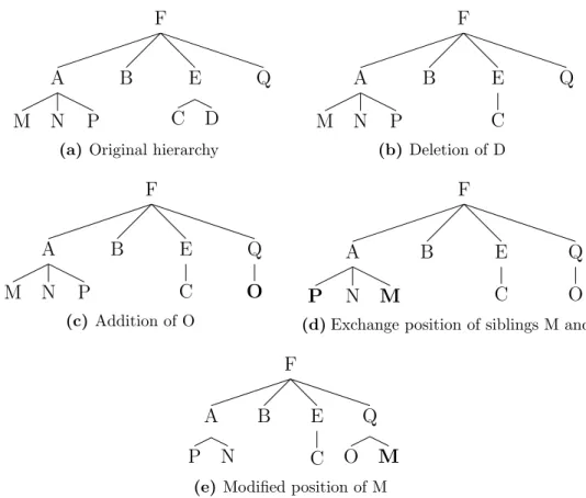
that are just moved to another part of the hierarchy which is a typical phenomenon when restructuring or refactoring the software system. An illustration of such changes is shown in Figure 1.2. F A M N P B E C D Q

(a) Original hierarchy

F A M N P B E C Q (b) Deletion of D F A M N P B E C Q O (c) Addition of O F A P N M B E C Q O

(d)Exchange position of siblings M and P F A P N B E C Q O M

(e) Modified position of M

Figure 1.2: The changes of a hierarchical organization

Telea and Auber [31] have already introduced a system that deals with software systems that illustrate the changes discussed above. Their work focuses on changes of source code overtime whereas the proposed visualization tool is able to work with any kind of evolving hierarchical data.

Hierarchical data can become large in many dimensions depending on the application domain. In software development for example we may have to deal with several million elements on the source code level and several thousand time steps depending on the granularity of the analyzed time interval.

An exploration of the raw textual data is hence a very time-consuming process if not impossible at all. For this reason, visualization is applied to such time-varying hierarchical datasets with the goal to find as many insights in the data as efficient as possible by exploring the perceptual abilities of the human visual system and the strengths for pattern recognition.

(15)

1.2

Aim of the Project

Hierarchical datasets can be found in many application domains where a large number of items (files, products, employees, stocks, etc.) can be handled and managed more efficiently when they are grouped into larger entities.

Nowadays, huge amounts of data are stored in databases, archives and even clouds, so this makes it important for the person in need of a specific information extracted from a huge pile of data to have an easy user friendly tool that helps visualizing certain data depending on user specifications and needs. Hospitals for example, have large amounts of files storing patients’ medical history along with their personal information. Being able to keep track of all these information and keep track of changes is a tiring and challenging process. Changes mentioned could be like having data moved, deleted or added which a↵ects the hierarchy of files and folders. Hence the importance of hierarchy comparison is required.

Small hierarchical structures are very e↵ective to locate information, but the content and organization of large structures is much harder to grasp. So in such cases the visual-ization of large hierarchical datasets is an important topic in the visualvisual-ization community.

Comparison of hierarchical information is of importance within various areas; for ex-ample, evolutionary biology, human resources and personnel, software development and hospitals as mentioned above [35]. Since human vision is sensitive to patterns, variation of colors and shapes we can have answers to specific questions very quickly. So visualiza-tion allows us to focus only on informavisualiza-tion that is important such as trends and outliers.

The aim of this project is to implement a tool that is capable of visualizing and interacting with large amounts of data in a user friendly manner to have a better and faster understanding of the data. To this end there are many visualization techniques for visualizing and analyzing large datasets. In this thesis we apply the approach of Indented Pixel Tree Plots (IPTPs) as the technique for analyzing dynamic hierarchies since it provides a scalable variant for visualizing hierarchies and allows good comparisons between time steps by aligning the plots side-by-side.

1.3

Remainder Of The Master Thesis

This thesis consists of the following chapters. Chapter 2 discusses the State of the art in visualizing hierarchical datasets, explaining the di↵erent techniques for exploring

(16)

large amount of information as well as the di↵erent methods of dynamic visualization and how to preserve the mental map. Followed by Chapter 3 describing the datasets used for user testing and the insight gained after visualizing them. In Chapter 4, the project architecture is described embracing the process overview, the class diagram and the features and functionalities introduced by the tool. Chapter 5 discusses the implementation of all algorithms and methods and describes the Graphical User Interface (GUI) of the tool. Finally, Chapter 6 contains the conclusion, the limitations and provides possible directions for future work.

(17)

Chapter 2

State Of The Art

(a) Node-link dia-gram

(b) Treemap (c) Layered icicle plot

(d) Indented outline

Figure 2.1: Visual metaphors for representing hierarchical data: (a)Node-link diagram. (b)Treemap. (c) Layered icicle plot. (d) Indented outline.

There is more than one method of hierarchy visualization available nowadays so it would be more e↵ective to have them organized into categories. The first category contains node-link diagrams, the second nested enclosure techniques (space-filling technique [6]) like the Treemap, the third category the stacking approaches (Layered icicles), leaving the indented outline style in the fourth category, see Figure 2.1(a)-(d). Even though each category has its own advantages and disadvantages the only identification of perfection of such a category can be investigated by conducting comparative user studies for di↵erent user tasks that needs to get accomplished using the di↵erent categories mentioned.

2.1

Hierarchy Visualization Systems

Since the hierarchical data structure has been widely used specially in the Information Visualization area [19], the most common structure would be the tree-like (node-link) structure and it can be used in the visualization of file system, organizational charts,

(18)

web sites, decision trees, genealogy and digital libraries. Even though such a structure is widely used and various layout algorithms have been developed as well the main problem there is the efficiency of conveying the topological structure of large trees when visualized. The main purpose of the visualization techniques proposed is to solve problems asso-ciated with hierarchy visualization techniques, i.e., such problems could be as follows:

• Using efficiently the available display space while conveying the complete hierarchi-cal structure

• Allowing the user to examine details of various regions of the hierarchy simultane-ously

• Enabling the user to easily interact with the hierarchy and perform tasks such as modifying the hierarchy and selecting nodes on which to perform operations

Despite the various advantages of those techniques, however, neither one of them can solve all the problems whereas most recent hierarchy visualization research focused on the challenge of displaying large hierarchies in an easily comprehended form.

2.1.1

Node-link diagrams

The node-link diagram (NLD) represented in Figure 2.1(a), is probably the most natural way to display nesting structures [23]. It is the most familiar diagram to users and it is appropriate for displaying the shape and structure of a tree. However, it fails to scale for large datasets. Node-link diagrams are suited better for showing the di↵erent levels and depths of a hierarchical structure. For example, Battista et al. [5], and Reingold and Tilford [23] use conventional node-link diagrams to depict relationships between hierarchically ordered elements. The node-link visual metaphor is considered the most widely used, well-established, de-facto standard for hierarchy visualization [2].

Node-link diagrams convey a clear and unambiguous structure of nodes. The parent-child relationship is represented using links and elements which are presented as nodes. However, node-link diagrams distribute nodes unevenly, leaving upper level nodes sepa-rated by white space, and lower nodes densely packed. While node-link diagrams show nesting structures very clearly, they consume screen space inefficiently, and do not scale well for large datasets. This means they are only beneficial when small trees need to get displayed, as a result many approaches have been proposed to supplement the node-link diagrams. The well-known alternatives include Treemaps, cone trees, and the hyperbolic browser [38].

(19)

Figure 2.2: Node-link diagram [38]

2.1.2

Treemaps

Treemaps are enclosure diagrams belonging to the space-filling techniques. Instead of using adjacency or node-link for hierarchy representation they use the concept of con-tainment as a visual metaphor [12].

Variants of Treemaps

The most common way to visualize hierarchies is by using trees, where edges describe the parent-child relationship between nodes [16]. However, Treemaps utilize a more space-constrained technique to visualize hierarchies, which solves the problem of normal trees having lots of non-utilized display area [3]. This is by displaying nested sequences of rectangles, whose areas represent the attributes of the dataset, hence allowing an easier comparison of node sizes. This implies that Treemaps fall under the nested containment category (Figure 2.1(b)). This category di↵ers from the three other categories where child nodes are drawn inside parent nodes, however they are represented outside in the other forms, whereas shades of colors represent the depth of each attribute. Treemaps are space-efficient [25] and perform well at giving an overview of very large trees, visu-alizing thousands of nodes constructing a hierarchical dataset [6]. However, and unlike node-link methods, it does not allow a clear node structure representation, especially when visualizing a balanced tree where all parents have the same number of children and leaves have same node sizes as this results in a treemap having the form of a regular grid. This unclear structure makes the di↵erent levels of the tree harder to perceive and distinguish. Only leaf nodes are clearly perceived since they overlap the parents’ areas. This drawback makes it less familiar to users than the node-link technique since it could be more difficult to interpret a hierarchy unambiguously.

(20)

(a) (b) (c)

Figure 2.3: Di↵erent Treemap layouts: (a)Slice-and-dice. (b)Squarified. (c)Pivot by split size [28].

There are several algorithms to create treemaps [34, 28, 25, 7, 33, 32]. The original treemap layout is called slice-and-dice [Shneiderman 1992], illustrated in Figure 2.3(a). It employs parallel long lines to divide a rectangle representing an item into smaller thin elongated rectangles representing its children [25]. The orientation of the line is switched from horizontal to vertical and vice versa, whenever a new level is introduced. Despite the algorithm’s simplicity, the long skinny rectangle lines with a high aspect ratio between width and height could be sometimes harder to recognize, select and compare in size and label.

Treemaps have been widely used in many domains starting from financial analysis to sports reporting [25] like visualization of a tennis match [27] as well as in mainstream me-dia, such as in displaying news headlines. However, an unexpected advantage of treemaps is the ease at which shallow nodes can be seen no matter how deep the subtree under a node may be, since treemaps tend to allocate more screen space to shallow nodes.

Squarified Treemaps

As an alternative, a ”squarified” treemap algorithm [7], illustrated in Figure 2.3(b) in-troduced by Jarke van Wijk, and a ”cluster” treemap method in Figure 2.3(c), described in Wattenberg having simple recursive algorithms, were introduced to reduce the overall aspect ratios to have the long skinny rectangles refined to square-shaped with aspect ra-tios close to one for better node detection and comparison [25]. Although these methods presented a clear refinement from the aspect ratio point of view, they sometimes lack the clear hierarchy structure preserved in the original slice-and-dice layout. Other known drawbacks [28] reported are that changes in the dataset can cause dramatic discontinuous changes in the layouts produced by both cluster and squarified treemaps. The second drawback of these layouts is that they cannot retain the given order of data, while many datasets contain ordering information that is helpful for seeing and distinguishing certain

(21)

patterns or for locating particular objects in the layout.

Ordered Treemaps

Ordered treemaps [28] were then introduced to address the drawbacks of the cluster and squarified methods presented previously. The ordered treemaps algorithm ensures that nodes near each other will in fact, be placed close to each other in the layout. Hence, they preserve the order of nodes displayed while keeping the aspect ratio as low as possible. Moreover, they provide a smooth change in the treemap layout when data is dynamically changing over time (data is getting updated), so it is easier for long-term users to recognize nodes being displayed and to easily allocate them.

Nested Treemaps

A small remedy developed to overcome the challenges of the treemap layout were the nested treemaps [16]. Instead of having the rectangle subdivided into smaller rectangles, a new rectangle is drawn inside the parent rectangle, and in turn, is subdivided into smaller rectangles representing the child nodes. This results in each group of siblings being enclosed in a margin which facilitates the recognition of parent nodes and layout structure. However, when the hierarchy is getting deeper, it requires more e↵ort to view it easily.

Figure 2.4: Nested Treemap [12]

Cushion Treemaps

In order to provide the users with a better representation of the visualized structure of the treemap, cushion treemaps [33] were brought out. This type of treemaps uses shading

(22)

to provide an easier interpretation of the hierarchical structure, since human perception of shades variation is shown to be very fast [15].

Figure 2.5: Cushion Treemap [33]

Pebble Treemaps

Figure 2.6: Pebble Treemap [36]

”Pebble Treemaps” also known as ”Circular Treemaps” or ”Radial space-filling” tech-nique, is a nested circles representation introduced by Wetzel [36], as a refinement to the rectangular treemaps. This approach can better reveal the hierarchy structure and achieve an aspect ratio close to one. However, this approach does not utilize space as efficiently as the rectangular-shaped treemaps and a circle size does not reflect the element (file) but it represents its size.

(23)

Colorizing of circles can di↵er depending on certain attributes. For instance, Wetzel represented a directory in which di↵erent files and circles were coloured depending on the file type (images, documents, etc.) as shown in Figure 2.6.

Voronoi Treemaps

Figure 2.7: Voronoi Treemap [3]

All treemaps described above are restricted to axis-aligned rectangles in their repre-sentation. Balzer et al. [3] developed a variation of the treemap algorithm which utilizes arbitrary polygons such as triangles and circles as shown in Figure 2.7 instead of rectan-gular shapes. Its advantages are that the aspect ratio between width and height is closer to one where treemaps lack such advantage, another upside of that structure is that there are no overlappings of nodes and boundaries between hierarchy levels and can be notably observed leading the structure to be better identified 1_.

The nodes in the hierarchy levels are represented by a set of polygons which forms a treemap layout at the end. Polygons support the usage of Voronoi tessellations 2 _for their subdivisions [4].

2.1.3

Layered icicle

A layered icicle diagram proposed by Kruskal and Landwehr [18], uses a space-filling visualization like a treemap. There are two styles reported in literature that represent this diagram: a ’Cartesian style’ and a ’Radial style’. A description for both styles is provided next.

(24)

Figure 2.8: Cartesian layout [12]

Cartesian style

Icicle layout is very similar to the node-link diagram in that the root node is always placed on top, having its child nodes underneath. The main di↵erence is that rather than presenting the parent-child relationship using links, nodes are drawn using solid shapes, either arcs or bars and their placement in adjacency to other nodes in the hierarchy indicates their position [12].

Icicle trees [22] are very space-efficient, and have a well-organized hierarchical struc-ture that can be easily understood and seen since its strucstruc-ture is very similar to normal tree structures which is very familiar to users. Their structure is simple and easy; child nodes are positioned under their parents in the same manner a normal tree structure would position its children except that this type of tree has nodes with no links which makes it more space-efficient than normal trees. Nodes are represented using rectangles. The root is displayed as a horizontal rectangle placed on top, and its children are also rectangles placed underneath the root rectangle. Child nodes are placed under their parents in the same manner. The length of all rectangles representing the children of a specific parent rectangle of a node can never exceed the parent node length.

One shortcoming of this display concept is how to step down the tree where the rectangles keep getting smaller. This makes it a bit challenging to navigate through these dense areas. Moreover, some nodes take up more space than required, like the root node which takes up as much space as the sum of all its children.

1_{http://infosthetics.com/archives/2006/01/voronoi treemap data visualization.html}

(25)

Radial style

This is another type of ”Icicle Layout”, but with a circular representation. This rep-resentation is also called ”Sunburst Layout”. In this layout, attributes constituting the hierarchy are arranged in a radial form, where the root element positioned on top of the hierarchy is placed at the center and deeper levels are placed farther away from the center. The size of an element is represented by the angle it subtends, hence, the bigger its size the wider the angle. Color for each element can be given to represent the element type if we are representing a file directory for instance [29]. An example of this layout is shown in Figure 2.9.

Figure 2.9: Sunburst layout [12]

Radial space-filling (RSF) diagrams [13, 5] compromise between space-efficiency uti-lization while maintaining the topological tree structure visibility. Evaluations held by Stasko and Zhang [29] using their RSF tool, ”Sunburst”, proved the ability of RSF in conveying the tree structure over treemaps. However, an RSF technique fails to capture the details for nodes with high depth level values, and when the hierarchy is large, the small slices are hard to determine. Focus+context techniques are used to overcome these drawbacks as will be described shortly.

Three methods were introduced to overcome these limitations and explore small parts of the hierarchy displayed. Andrew’s and Heidegger’s two semi-circular approaches [1], Stasko and Zhang’s angular detail, detail outside, and detail inside approaches [30], which presents an enhancement of Andrew’s approach, aim to overcome the discussed limita-tions. At last, InterRing that was presented by Yang et al. [37] in 2003 to tackle the drawbacks of both mechanisms is another method. An explanation of all three methods will follow next.

(26)

Information slices

The Information slices approach is a visualization technique introduced by Andrews et al. [1] to visualize and manipulate large hierarchical data. Information is represented using semi-circular discs. Di↵erent discs represent multiple levels where higher depth levels are always placed at the periphery of the semi-circle. Figure 2.10 shows a prototype of information slices they implemented for visualizing the hierarchical tree structure of a file system.

Figure 2.10: Information slices [1]

This approach allows the user to expand a certain area on the displayed hierarchy. Two discs can only be shown at once; further expanding removes the leftmost disc from the main panel and is only shown as an icon and the new expansion is observed at the right.

The user is also able to set some configurations such as how many levels to display on each disc, or to display children in which order, i.e., alphabetical or by size.

Focus+Context

Three methods were proposed to have a smoother and more flexible alternation between global and detailed hierarchy display than Andrew’s and Heidegger’s semi-circular ap-proach. The techniques are similar in that by clicking on an item, it is focused and observed in the same display of the entire hierarchy. Nevertheless, they di↵er in how they display the focused area. Each has its own advantages and drawbacks. The three methods are as follows [30]:

(27)

• Angular detail method: The entire hierarchy shrinks and is moved to the top right corner of the display screen, and the item selected is focused and placed at the center of the display. This technique requires more space, although it looks natural to the user, see Figure 2.11 for clarification.

• Detail outside method: The overview shrinks at the center of the display while the selected item is enlarged and placed in form of a new circular ring around the overview.

• Detail inside method: The overview is shrunk and widens to have the focused area placed inside it, i.e., at the center of the overview.

Figure 2.11: Sequence of frames from the Angular detail technique, allowing a viewer to focus on small peripheral files [30].

Despite the better observation of details these techniques o↵er, they su↵er from some drawbacks [37]. They cannnot preserve the user’s mental map (explained in the following chapter) because of the big visual shift on the original overview observed after an item is focused. Complex animation is needed in order to follow the changes operated on the original overview. They also do not use space as efficiently as the original RSF, and they cannot handle multiple foci.

InterRing

Previously described RSF techniques do not o↵er as many interactivity as o↵ered by tree nodes and text-based hierarchy visualization systems. Yang et al. [37] proposed a new

(28)

(a)Roll-up/Drill-down (b)Rotate (c)Zoom in/out

(d) Distort (e) Modify

Figure 2.12: Operations implemented for interactivity on hierarchical structures [37]

RSF technique ”InterRing” to enable users to visualize, modify, and perform selection on the hierarchy and to overcome the drawbacks of Stasko’s and Zhang’s three mechanisms discussed previously using a new distortion approach.

Operations implemented by InterRing for user interactions are as follows:

• Selection: The process of selecting multiple nodes for further processing, allows the user to isolate a set of nodes in the hierarchy that can then be highlighted, masked, moved, or deleted.

• Reconfiguration: The ability to adjust the hierarchical structure means that users can move a subcluster from one cluster and place it in another to improve the quality of the hierarchy.

• Drill-down/Roll-up: The process of exposing/hiding subhierarchies helps users to only show objects of interest and prevent other objects from showing.

• Pan, zoom, and rotation: The process of focus, scale, and orientation adjustment to the hierarchy currently on display allows panning and zooming, meaning that users can enlarge the context displayed and examine the details of the hierarchy. Rotating allows users to rotate clusters of interest to specific angles and avoids cluttering the labels of the selected clusters.

• Distortion: The process of enlarging certain parts of the hierarchy without a↵ ect-ing the context of the total display. It allows users to have multiple foci, provides

(29)

an easy way to follow changes and does not need extra space for the focus+context display.

2.1.4

Indented layout

Indented tree layouts are used excessively by operating systems to represent file directo-ries. They place all items along vertically spaced rows and use indentation to represent the parent-child relationships. Windows Explorer is a classical example of a tree outline structure as shown in Figure 2.13.

Figure 2.13: Windows Explorer [22]

An indented outline structure also allows efficient interactive exploration of the tree to find specific nodes. Despite the big vertical space needed for visualizing the hierarchy, the positioning of nodes separately on horizontal lines makes it beneficial to add information to the right of each corresponding node [12].

Indented Pixel Tree Plots (IPTPs), a new hierarchical tree visualization introduced by Burch et al. [8, 9] is a technique that is based on the visual metaphor of indented outlines present in graphical file browsers and everyday software developers’ source code. The fact that indented outline approaches are popular in file browsers such as Microsoft Explorer makes it familiar to the user to understand and easily read the hierarchy representing the data [8].

The IPTPs are in a way similar to reading a text fragment where it must be read from left to right to understand the hierarchical semantics, hence they are labeled as a one-and-a-half dimensional visualization approach [8].

(30)

IPTP representation

IPTPs represent inner vertices using vertical lines and employ horizontal lines to rep-resent leaf vertices. Each horizontal line reprep-resents a di↵erent level. Each node in the hierarchy can be mapped to a certain horizontal line according to its tree level. Edges are represented only implicitly by the vertically and horizontally aligned structure of the plot. Adding edges would be considered superfluous as Tufte mentioned - unneeded in-formation that by discarding, would not a↵ect the understandability and readability of the graph. Parent-child relationships are expressed by indentation of the corresponding geometric shapes with respect to the hierarchical levels of the respective parent and child vertices.

Figure 2.14: Indented pixel tree plot [9]

A user study was conducted by Burch et al. [8] to investigate the readability of an IPTP in comparison with a node-link diagram (NLD), - also known as the de-facto standard for hierarchy visualization - in a static way, without colour gradient and any interactive features. The experiment was performed in a laboratory that isolates any distractions, and had been applied on 30 participants. These participants were a mixture of males and females of computer science and engineering backgrounds. Some of them had some background on the concept of visualization techniques and some had not heard of it yet. All participants were tested to ensure they have normal colour vision. Each participant was assigned three tasks. The tasks assigned are described as follows:

• T1: Finding the least common ancestor of two leaf vertices

• T2: Checking if elsewhere in a plot there exists an identical subhierarchy

• T3: Estimating the larger subhierarchy

Prior to the experiment, a 10 minutes training was done to the participants to assure their understanding on both techniques, IPTPs and NLDs. Then, an average of 15 minutes was given to each participant in the evaluation and each of them had to perform all 3 tasks using both techniques (IPTPs and NLDs) with seven trials with di↵erent datasets (di↵erent tree sizes). After finalizing the tests, participants were given the opportunity to identify their preferred technique by filling in a questionnaire.

(31)

The results of the study conducted were analyzed over all dataset sizes applied on all three tasks. The analysis was performed from di↵erent perspectives. Completion time, accuracy and the overall preference for each participant, were the perspectives taken. Concerning the completion times, it was found that in tasks T1 and T2, the average time taken to complete both techniques was similar, no significant di↵erence. The significance di↵ered in T3, where it was found that for small and large datasets NLDs were faster to read while for medium sized datasets, IPTPs had very high significance. The aver-age calculated indicated that neither of both techniques was significant in that concern. Concerning the accuracy, statistics shows that no significance was found. Regarding par-ticipant’s overall preference, it was found that for small datasets, participants preferred the node-link diagram and for large datasets IPTP was found to be more useful.

Andrews et al. [2] also conducted a user study to compare four hierarchy browsers which are the Windows Explorer style tree view, the information pyramids, the treemap and the hyperbolic browser. Task analysis was performed which involved 32 test users where each user performed eight tasks on each browser. Task completion time, subjec-tive ratings and overall preference data were collected. Despite having no significant di↵erences in performance, users significantly preferred the tree view browser.

2.1.5

Hybrid Representation

There are also some visualization techniques that use a combination of node-link and treemaps methods like ”elastic hierarchies” [38] and ”space-optimized tree visualization” [21]. These techniques o↵er a trade-o↵ between the space-efficiency that characterizes the treemaps and the clear structure display o↵ered by the node-link diagram.

Elastic hierarchy

An elastic hierarchy allows users to examine the content of a treemap in more detail and select nodes within it more easily. It also allows the user to change the representation of the hierarchy at any time. Accordingly, this hybrid representation has the potential to flexibly combine the familiarity and clarity of node-link diagrams with the space savings of treemaps. Selection within a treemap is usually difficult because internal nodes are covered by their descendants. Elastic hierarchies solve that problem by implementing a selection technique by showing several tabs to select from corresponding to di↵erent levels in the treemap. Each tab causes its level to highlight and allows the users to examine the nodes at that level.

(32)

Figure 2.15: Elastic hierarchy [38]

2.2

Technique for changing hierarchical data

Code Flows [31], a visualization technique for analyzing source code structure evolution, uses a vertical icicle plot where nodes are ordered by the order of the code lines in the file to show the layout of the desired source code file. It uses tubes to connect two matched nodes in two successive versions. To follow the entire evolution of a particular code fragment for example, a code swap can be easily detected by crossing tubes. The visualization techniques are implemented using the Tulip visualization framework.

2.3

Time-Series Visualization

Time-series data can be visualized in many ways. The most important visualization techniques for time-series data are sequence charts, point charts, bar charts, line graphs, and circle graphs.

2.3.1

Animation vs. Static

Dynamic hierarchies can be visualized in two ways, either by animation or by present-ing the change uspresent-ing successive diagrams. The drawback uspresent-ing animation to visualize dynamic hierarchies is that the core diagram gets lost and we can’t keep track of what exactly has changed, especially when we need to keep track of data in various timesteps. The mental map can therefore be lost which may lead to misinterpretations, as will be discussed thoroughly in the next section. Examples of such hierarchies using animation to represent dynamic hierarchies, are information slices and InterRing as were explained in details in Section 2.1.

(33)

Static hierarchies on the other hand can keep track of all changes during di↵erent time intervals, by displaying the di↵erent hierarchies successively against each other. Colors or lines can be added to visualize the changes. This remedies the misinterpretation and preserves the original hierarchy structures in all times.

In our project, static hierarchies are used to visualize the dynamic hierarchies over time and lines are used with di↵erent colour codes to visualize the changes.

2.3.2

Mental Map

Since humans easily memorize pictures, graphs, maps, etc. basically anything that is sketched or visualized, so information represented in any of these formats can be easily retrieved from the brain. People usually describe a location of a given place for example from a virtual graph they visualize in their heads3_{, the person’s perception of that image} is known as ”mental map”4_.

In dynamic hierarchies, rearrangements of some nodes can occur, as well as the re-moval and addition of new nodes [20]. For example an added node can overlap an existing node which can also e↵ect the reposition of other nodes, this can e↵ect the user’s mental map on the original diagram structure. The mental map of the user should be preserved for ease of understanding on how the hierarchy structure has changed over time [11]. Otherwise, if the mental map was lost the viewer would take one object for the other over time and consequently makes misinterpretations.

In this project we visualize dynamic hierarchies while preserving the mental map [10], by implementing a static diagram and illustrating the changes applied to hierarchies like added, removed or moved nodes, using coloured lines, maintaining the basic hierarchy structure. Lines demonstrate the change by having its start point where the node was located in the previous hierarchy, and its end point where it is located in the successor hierarchy. Lines are coloured to express di↵erent meanings; ”red” is to represent removed nodes, ”green” to represent added nodes and ”blue” to express moved nodes, see an illustration for clarification in Figure 2.16.

3_{http://www.fedstats.gov/kids/mapstats/concepts mentalmaps.html}

4_{A mental map is an individual’s own internal map (person’s personal point-of-view perception) of} their known world. http://geography.about.com/cs/culturalgeography/a/mentalmaps.htm

(34)

(35)

Chapter 3

Case Studies

To illustrate and test our application and demonstrate the usefulness of IPTPs, we ap-plied the IPTP technique to several datasets. We investigate very large datasets such as the National Center for Biotechnology Information (NCBI) taxonomy that contains several hundred thousand nodes (324,000 nodes) representing the names of all organisms that are represented in the NCBI genetic databases with at least one nucleotide or protein sequence [24]. This huge file was understandable from the IPTP representation, which may be difficult when the same dataset is visualized in a treemap, a layered icicle plot, or a node-link diagram due to visual scalability reasons. Furthermore, the plot can be scaled down immensely and the hierarchical structure still remains visible. Figure 3.1 illustrates the IPTP representing the NCBI taxonomy dataset where subhierarchy selec-tion is applied - shown by the yellow triangles - until reaching a detailed view. From the overall view of the dataset represented in Figure 3.2, we can easily detect the deepest part of the IPTP as highlighted by the blue rectangle for example. This is easily grasped since we know that green nodes represent the leaf nodes and the higher the depth level it gets, the more it is indented to the right.

The only problem with the NCBI dataset is the long time it takes for the IPTPs to get plotted and to adopt to whatever action is taken on them.

Another kind of datasets were used for testing and demonstrating dynamic hierarchies. They represent the evolving prefix tree structure of words occurring in paper titles. All papers from the field of computer science are collected for each year. Then these are preprocessed to generate a prefix tree for each year. The data comes from the DataBase systems and Logic Programming (DBLP)1 _{and is given in an XML file.}

(36)

Figure 3.1: IPTP representing the ’NCBI taxonomy’ highlighting a subregion

Two DBLP datasets were tested, a small DBLP consisting of 100 elements with a maximum depth of 4 ’dblp.newick.100’, meaning it is not very deep but it consists of many timesteps. The other dataset is bigger than the first one with up to 1,000 elements with a maximum depth of 4, ’dblp.newick.1000’. The hierarchies start with small numbers of elements and get bigger over time. For example, in the year 1949, there are only 145 elements and in 1974 the size of the file reached 1,000 elements.

All datasets are represented in newick file format2_{, which will be explained later in} 2_{Newick tree format is a way of representing graph-theoretical trees with edge lengths using} paren-theses and commas.

(37)

Figure 3.2: IPTP representing the ’NCBI taxonomy’ illustrating the deepest leaf nodes (en-closed by the blue rectangle)

Chapter 6. The evaluation of the tool with all its features and functionalities were done on the ’dblp.newick.100’file as will be discussed.

The dataset in use represents data from 1936 until 2012. Since the display area can only take 10 IPTPs, analysis and evaluation will be discussed on a 10 IPTP view.

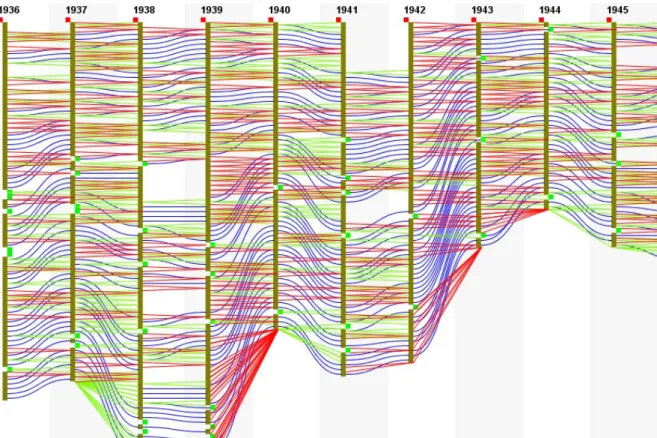
Figure 3.3 represents IPTPs from 1936 until 1945. Depth can easily be depicted by the di↵erent colors given to each depth level as can be observed by the Hierarchy Legend as shown in Figure 3.4

After comparing the IPTPs displayed as shown in Figure 3.5 we start analyzing how hierarchies evolved over time using the coloured lines knowing that red lines represent

(38)

re-Figure 3.3: IPTPs of the ’dblp.newick.100’ file

Figure 3.4: Hierarchy Legend

moved nodes, green lines represent added nodes and blue lines represent changed position nodes.

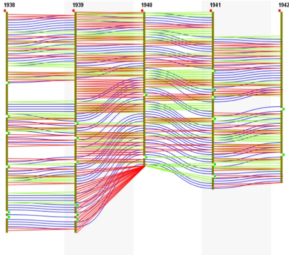
To better understand the changes, we illustrate some of the tool’s features like filtering and searching and analyze our observation. Figure 3.6 represents the IPTPs after applying 2 filters, the first is to filter only nodes starting with alphabet ’a’ and the second is to filter nodes starting with alphabet ’p’. From the observation, we can clearly see that from year 1941 to year 1942 there wasn’t any removed, added or changing position nodes. As for the nodes starting with the alphabet ’p’, we can see that from 1944 to 1945 the nodes only changed positions in the hierarchy.

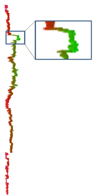
To have a look at a specific node and observe the changes, ’Searching’ is applied. For example in Figure 3.7 we can observe and keep track of changes on a node called

(39)

Figure 3.5: IPTPs of the ’dblp.newick.100’ file after comparison

’boolean’. We can see that it was added in 1937 and removed in 1939, then reappeared in 1945.

Knowing that the system can display a large number of files consecutively, in order to gain insight on specific hierarchies at certain timestamps, we use the time filter to choose the hierarchies we are in need to analyze. We give a start date and an end date of hierarchies to display. Figure 3.8 shows IPTPs starting from 1940 until 1948 according to the user selection of dates. So instead of searching all along the huge number of files, time filter as shown makes analysis easier when in need of observing changes at specific timings.

Keeping track of only added nodes or removed nodes is also an easy task. Predefined filters are implemented and can be chosen from a drop down list. Figure 3.9 is an example of IPTPs after applying the time filter and choosing to only show added nodes (represented using green lines) on only nodes starting with the character ’a’ as well as on the node named ”arithmetic” (represented in yellow). As can be observed from Figure 3.9, in years 1942 and 1943 neither node starting with alphabet ’a’ nor ’arithmetic’ is newly added. Observing the IPTPs we can analyze that since 1940 ’arithmetic’ was added in 1945, changed position in 1946, removed in 1947, and reappeared in 1948.

(40)

Figure 3.6: IPTPs of the ’dblp.newick.100’ file after applying filters

nodes which then displays a tooltip with the node name. As seen in Figure 3.9, ”axiom” is the node hovered.

The analyses above are all made by IPTPs observation and by applying di↵erent types of filters for better investigation. Other analyses can be made by observing the statistics displayed - as seen in Figure 3.10 - after IPTPs selection, which demonstrates the changes in percentage between IPTPs, like how many nodes were added, removed or changed positions. This is shown by the red rectangle in Figure 3.10, which illustrates the changes between IPTPs of years 1936 and 1937: 26% of nodes were added, 31% were removed, and 52% changed positions in 1937. The Figure also highlights another blue rectangle that demonstrates file details of the year 1936, we can see that it contains 80 nodes and a maximum depth level of 4. This information changes accordingly whenever an IPTP is selected.

(41)

Figure 3.7: IPTPs of the ’dblp.newick.100’ file after searching the element ’boolean’

(42)

Figure 3.9: IPTPs of the ’dblp.newick.100’ file after applying the time filter, and show only alphabet starting with ’a’ as well as the result of a search on ”arithmetic” (shown in yellow)

(43)

Figure 3.10: General information about IPTP of 1936 (blue rectangle) and changes between IPTPs of years 1936 and 1937 (red rectangle)

(44)

(45)

Chapter 4

Project Architecture

4.1

Process Overview

This section gives an insight about the process of visualizing IPTPs and how they evolve over time. This process can be sub-divided to multiple steps as can be viewed in Figure 4.1.

Figure 4.1: Process overview diagram

First, we use a newick file parser to extract a hierarchical tree structure Ti consisting of nodes from every newick file versionfiof the files contained in the directory of interest. Second, we display the hierarchies (IPTPs) corresponding to the parsed files. Third, a comparison takes place and we use the ”Comparison Algorithm” described thoroughly in Section 6.4 to detect the changes between consecutive hierarchical structures Ti, Ti+ 1. Fourth, we draw links between consecutive hierarchy nodes to represent and illustrate the

(46)

changes calculated in the previous step. Many interactive features can then be applied on the hierarchies visualized for a better understanding, discussed in Section 5.3 where we will describe each step in detail and how they were implemented in Chapter 6.

4.2

Class Diagram

In order to best illustrate the interdependencies and relationships among the di↵erent system modules, we thought it was best practice to create a class diagram. The here-under depicted Figures 4.2 and 4.3 define the overall static view of the system, where a description of how each class (together with it’s associated attributes) relate to every other class present in the system.

(47)

(48)

! Li ne D et ail s! +l in eT yp e: !S tr in g! +n od eI nf o: !N od eS ta tu s! +p at hl in e: !P at h2D ! +l in e: !L in e2D ! Ne w ic kF ile Pa rs er ! @pa rs e( St ri ng ): !N od e! @pa rs e( St ri ng !s ,!N od e! pa re nt ): !N od e! @ge tD ep th () :!i nt ! +! s! :!S tr in g! +! in de x: !in t!! =! 0! +! co un tN od es :!i nt !!=! 1! +! di sc ov er ed N od es !:! Ar ra yL is t< N od e> ! No de ! @ se tN am e( St ri ng ): !v oi d! @ge tN am e( ): !S tr in g! @nu m Ch ild re n( ): !in t! @ad dC hi ld (N ode !n ): !v oi d! @ge tC hi ld (i nt !i) :!N od e! @ad dP ar en t( N ode !p ): !v oi d! @ge tP ar en t( ): !N od e! @ge tE xp an dC ur rV al ue () :! bo ol ea n! @!ge tE xp an dP re vV al ue () :! bo ol ea n! @to gg le Ex pa nd Cu rr en t! (N od e! n): !v oi d! ! +! na m e: !S tr in g! +! pa re nt :!N od e! +! le ve lV al ue !:! in t!! =! 0! +! ex pa nd Pr ev :!! !!! bo ol ea n! =t ru e! +e xp an dC ur r: !! !!bo ol ea n! =! tru e! +! ch ild V ec :! !Ve ct or <N od e> ! Ba rc ha rt Pa ne l! @!se tV al ue s( ): !v oi d! @!pa in tC om po ne nt !! (G ra ph ic s) :!v oi d! @se tF ile N am es () :!v oi d ! ! +! w id th :!i nt ! +! xP os it io n: !in t! +! m ax :!i nt !! +! nu m O fH ie ra rc hi es :!! !!! No de ![] [] ! +d iv id eP an el :!i nt !! +! to tb ar s: ! Ar ra yL is t ! +a rr ay O fF ile s: ! Ar ra yL is t< Fi le >! +! sw it ch Li st :! Ar ra yL is t< In te ge r> ! +! re m ov eL is t: ! Ar ra yL is t< In te ge r> ! +! ne w Li st :! Ar ra yL is t< In te ge r> ! Ba rs O bje ct ! +! xP os :!i nt ! +n um O fN od es 1: !in t! +! nu m O fN od es 2: !in t! +n um R :!i nt ! +! nu m G :!i nt ! +n um B :!i nt ! ! Dr aw ! @se tH ash ta bl eO fS ub re gi on (i nt ! fi le N um ): !v oi d! @pa in tC om po ne nt (G ra ph ic s) :!v oi d! +a rr ay O fF ile s: !A rr ay Li st <F ile >! +a rr ay O fG ra ph s: !N od e[ ][ ]! +n fp :!A rr ay Li st <N ew ic kF ileP ar ser >! +t lp :! Ar ra yL is t< T ra ns la te Li st sT oP oi nt s> ! +l is tO fG ra ph Po in ts :! Ar ra yL is t< Po in t> ! +t ot al Li st O fL in es :! Ha sh ta bl e >! +t ot al Li st O fRe ct an gl es :! Ha sh ta bl e >! +c ho se nRe ct an gl es :! Ha sh ta bl e >! +d iv id eT im eF ilt er Pa ne l:! in t!=! 0! +s ub re gi on :!b oo le an !=! tr ue ! +p ix el Si ze :!d ou bl e! +r ec t: !Re ct an gl e2D ! +R :!i nt ! +G :!i nt ! +B :!i nt ! +n oO fL ev el s: !in t! +! le ve ln :!i nt ! +l ev el p: !in t! +n od eW :in t! +n od eH :in t! ! IP T Pt ool ! @ se tT oo lb ar () :!v oi d! @se tM en ub ar () :!v oi d! @op en D ir ec tor y( ):!v oi d! @co m pa re () :!v oi d! @cl ea rP an el () :!v oi d! @di sp lay In it ial V iew () :!v oi d! @cr ea te A nd Sho wG U I( ): !v oi d! ! +a rr ay O fF ile s: !A rr ay Li st <F ile >! +a rr ay O fG ra ph s: !N od e[ ][ ]! +n fp :! Ar ra yL is t< N ew ic kF ile Pa rs er >! +t lp :! Ar ra yL is t< T ra ns la te Li st sT oP oi nt s >! +lis tO fG ra ph Po in ts ! +c om pa re :b oo le an ! +c om pa re A ll: !b oo le an ! +n ew Pa ge :b oo le an ! +t im eF ilt er !:! bo ol ea n! +s ho w O ri gi na l:! bo ol ea n! +h ig hQ ua lit y: !b oo le an !

(49)

! Dr aw R ec t! *ad dR ec ta ng le( D ra w R ec t) :! vo id ! *ge tL is tO fR ec ta ng le () :! Ar ra yL is t< D ra w R ec t> ! *!ge tL is tO fR ec ta ng le s( ): ! vo id ! *se tL ist O fR ec ta ng le s! (A rr ay Li st <Dr aw R ec t> ): ! vo id ! *!a dd Le af (N od e!l ea f) :!v oi d! *!ge tL is tO fL ea f( ): ! Ar ra yLi st <N od e> ! *!ge tL is tO fL ea ve s( ): ! Ar ra yL is t< N od e> ! *!se tL ist O fL ea ve s! (A rr ay Li st <N od e> ): !v oi d! ! +!r ec t: !R ec ta ng le 2D ! +!n am e: !S tr in g! +!n od e: !N od e! +!A llL is tO fR ec ta ng le s: ! Ar ra yL is t< D ra w R ec t> ! +!L is tO fR ec ta ng le s: ! Ar ra yL is t< D ra w R ec t> ! +!l ea ve s: !A rr ay Li st <N od e> ! +!A llL eav es :! Ar ra yL is t< N od e> ! ! No de St at us ! +! no de :!N od e! +! no de N am e: !S tr in g! +! le ve lW as :!i nt ! +! le vel N ow :!i nt ! +! in de xW as :!i nt ! +i nd ex N ow :!i nt ! Di ff er en ce ! ! *che ck Le ve l( in t!in de xW as ,!in t! in de xN ow ): !v oid ! *!di ff er en ce B tw Fi les (N ode[ ]! No de sO fF ile 1, !No de [] !N od es O fF ile 2) :! vo id ! +! fo un d: !b oo le an !=! fa ls e! +! nu m Sw it ch ed :!i nt ! +! nu m A dd ed :!i nt ! +! nu m R em ov ed :!i nt ! +! sw it ch Li st :!A rr ay Li st <N od eS ta tu s> ! +! re m ov eL is t: ! Ar ra yL is t< N od eS ta tu s> ! +! ne w Lis t: !A rr ay Li st <N od eS ta tu s> ! +! co un ts Co m pa ri so n! Ar ra yL is t< Ca cu la te D iff er en ce >! +! de fa ul tC om pa ri so nP er c: ! Ca lc ul at eD if fe re nc e! +N od es O fF ile 1: !N od e[ ]! +! N od es O fF ile 2: !N od e[ ]! +n od e1: !N od e! +n od e2: !N od e! +f ile 1S iz e: !in t! +f ile 2S iz e: !in t! ! Ca lc ul at eD if fe re nc e! +c ou nt S: !in t! +c ou nt D :!i nt ! +c ou nt N :!i nt ! +! ad dP er c: !d ou bl e! +! ch an ge Pe rc :!d ou bl e! +r em ov ed Pe rc :!d ou bl e! +! pe rc en ta ge S: !S tr in g! +! pe rc en ta ge A :!S tr in g! +! pe rc en ta gR: !S tr in g! Do ub le Po in t! +x :!d ou bl e! +y :!d ou bl e! +x en d: !d ou bl e! +y en d: !d ou bl e! Tr an sl at eL is ts T oP oi nt s! *se tP oi nt s! (A rr ay Li st< N od eS ta tu s> ! ne w Li st ,!A rr ay Li st <N od eS ta tu s> ! de le teL is t,! Ar ra yL is t< N od eS ta tu s> ! sw it ch Li st ,!A rr ay Li st ! lis tO fG ra ph sP oi nts )! +! le ve lW as :!i nt ! +! le ve lN ow :!i nt ! +! in de xW as :!i nt ! +! in de xN ow :!in t! +! fa ct or :!i nt ! +! in de x: !in t! +! al l:! bo ol ea n! +! nL is t: !A rr ay Li st <N od eS ta tu s> ! +! dL is t: !A rr ay Li st <N od eS ta tu s> ! +! sL is t: !A rr ay Li st <N od eS ta tu s> ! +! pN ew :!A rr ay Li st <L in eP oi nt s> ! +! pD el et e: ! Ar ra yL is t< Li ne Po in ts >! +! pS w it ch :! Ar ra yL is t< Li ne Po in ts >! +! !fi le 1S iz e: !in t! +! fi le 2S iz e: !in t! +! no de Fr ac :!d ou bl e! ! ! Li ne Po in ts ! +P so ur ce 1: !D ou bl eP oi nt ! +P de st 1: !D ou bl eP oi nt ! +P so ur ce 2: !D ou bl eP oi nt ! +P de st 2: !D ou bl eP oi nt !

(50)

4.3

Features and Functionalities

Navigation and interaction facilities are essential in Information Visualization. Our tool is based on the visual information-seeking mantra: overview first, zoom and filter, then details-on-demand [26].

The tool supports a variety of interactive features to explore the hierarchical data such as collapsing and expanding specific nodes, getting information on a specific element and selecting a subregion for a hierarchy on a larger scale for better investigation. The tool’s features and functionalities are as follows:

- Region selection: Part of the indented plot can be selected by mouse pressed and mouse released functionality, highlighting a desired region. The selected region is then displayed at the right of the original hierarchy within a larger scale for a better observation.

Hierarchy expanding/collapsing: Using the mouse click functionality, clicking on a node representing an attribute can collapse or expand its corresponding chil-dren alternatively. So when a node is collapsed all its sub-nodes (chilchil-dren) are hidden, and whenever the node is expanded again the sub-nodes reappear.

-- Text pattern search: Typing in certain text in a searching browser, searches for the specified text in the indented plots displayed and highlights the corresponding nodes found.

- Zooming: A zoom in/out horizontal slider bar can be used for a larger/smaller scale on the indented plots displayed on the display screen for a more detailed representation or an overall view alternatively.

- Details-on-demand: Using a mouse over functionality, by moving the cursor on any element on the display screen, information is displayed as a tooltip at the current mouse cursor position. A tooltip could be placed either on a node element or a comparison line. A more detailed information for a specific element (node) like the node name, number of children of the node, the parent name and the depth is displayed as well on a text area shown on the tool’s right panel.

- High quality/Low quality (Resolution): For a faster rendering specially when representing huge datasets, the user can choose whether to display the indented plots with high quality (better resolution) with no aliasing or to have a bad quality plots rendered with aliasing.

(51)

- Interactive/Non-interactive (Display mode): The display mode can change whenever needed to either interactive or non-interactive mode. Meaning, if only a static view of the indented plots is needed with no interaction then the user can choose to switch to a non-interactive display mode which makes rendering faster. The user can change the display mode to interactive whenever needed. A static view is of importance when displaying huge hierarchies when there is no need of the interactive features, like only having the ability to scroll horizontally and vertically. - Filter: A list with some pre-defined filters is available on the tool’s left panel where the user can choose certain filter function like displaying only nodes that got added, on further hierarchies, or displaying only nodes starting with certain alphabet like ’a’ for example.

- Color coding: For a better visualisation of the di↵erent hierarchy levels, each level of nodes is represented in a di↵erent colour to distinguish it from other elements having other level values. So by user observation of the di↵erent colour gradients, user can easily identify the deeper levels from other shallow levels.

- Comparison: A comparison button is provided on the tool bar to provide and illustrate changes between consecutive hierarchies displayed. Colored lines are used to illustrate changes from one hierarchy to another.

- Delta (Percentage of change): Percentage of change on added, removed and changed position nodes between two consecutive hierarchies selected can be dis-played.

(52)

(53)

Chapter 5

Implementation

The following chapter gives a full explanation for the main building blocks of the tool. In order to help illustrate the ideas, additional descriptive elements including equations, figures and pseudocodes were also used when needed. The chapter starts by introducing

the Newick File Parser, which is responsible for the transformation and building of the

tree hierarchy from an input given as string. The Collapse/Expand Algorithm section describes how the node expansion and collapse is performed. Comparison algorithms are discussed in details next in the following chapter File Hierarchies Comparison. The visualization module is outlined in the subsequent section. The chapter encloses with the

IPTPtool section where the main method and GUI modules are implemented.

5.1

Newick File Parser

The main goal of this class is to parse the input file, that is given in Newick format. The ”Newick” format uses parentheses and commas to show the parent-child relationship to represent a hierarchy of data, e.g. (A,B,(C,D)E)F;. The tree representation of the newick file is shown in Figure 5.1.

F

A B E

C D

Figure 5.1: Tree representation of the parsed newick file ”(A,B,(C,D)E)F;”

As the edges don’t play a role in our file representation no processing on the edges en-countered during the traversal of the newick file is performed. TheNewickFileParseris implemented to traverse the parents and their children and record them in anArrayList

(54)

’discoveredNodes’ used for further processing throughout the application.

The file is read and stored in a String newickString that is then passed to the parser. The parser uses a recursive method to explore all the nodes. First, the parser extracts the root node knowing that it is placed at the end of the newickString be-fore the semicolon ’;’, and stores the rest of the newickString representing the root’s children. So in the example stated above, the root node will be F and its children will be A,B,(C,D)E. The parser then calls the recursive method taking as parameters the ’Parent’node (the root in this situation) and the’newickString’representing its chil-dren.

Before describing how the input string is processed and passed recursively to the method, the notion of bracket balancing and its benefits needs to be explained first. Bracket balancing simply aims at detecting the direct child nodes of the current parent nodes, and extracting the substring representing their sub-child nodes. In other words, the first direct child node to the current parent node is the first string after a perfectly balanced bracketing. The second direct child node to the current parent node is the first string after the second perfectly balanced bracketing, etc. Every direct child node detected is then recursively passed as parameter together with the preceding perfectly bal-anced substring to the same node to discover the nested child nodes. In order to achieve this, the input string is traversed from left to right character by character inspecting each one to determine its state. The perfect bracket balancing is being tracked by a variable called bracketcount. bracketcount is always incremented by 1 if an open bracket is encountered ’(’. In contrast it is decremented by 1 if a closed bracket is encountered ’)’. Any substring that is traversed while the bracketcount has a greater value than zero, is simply concatenated to form the string to be passed for the next recursive call. The first substring encountered while thebracketcountequals zero is treated as a direct child node for the current parent node, and passed recursively as a parent for the preceed-ing concatenated substrpreceed-ing (i.e. the substrpreceed-ing between the preceedpreceed-ing balanced brackets).

Before creating a new node the depth value of the node needs to be set. The root node is first initialised with a node depth value of 1 accordingly, all other nodes’ levels are set. If the new node being created is a child to the previous node created, then the depth level value associated with the previous node (the parent node) is incremented by one and assigned to the depth level value of the new node.

(55)

tree can then be calculated using the getDepth() method that gets the maximum node level stored from thediscoveredNodelist containing all created nodes resulting from the parsed newickString.

After parsing the newick file, the tree structure is then perceived. Since we are in need of an indented outline for hierarchy visualization, our implementation is a kind of a depth first search traversal.

parse(String s, Node root)

//s consists of only one child(one Node)

if is-simple-struct(s) then

return new Node(s); end

//complex structure

if !is-simple-struct(s) then

String bu↵er=” ”; //to store the String representing a Node’s children

for int i=0;i<s.length;i++ do

//when bracket count reaches zero

if is-balanced(charAt(i)) then

Node p=new Node(charAt(i));

root.addchild(p); //add node ’p’ as child to the parent ’root’

set-node-level(p); //depth level of node ’p’ is set to be equal to the parent node level+1

if bu↵er is not empty then

remove-outer-brackets(bu↵er); p.addchild(parse(bu↵er,p)); bu↵er=” ”; end end else

bu↵er=bu↵er+charAt(i); //if unbalanced bu↵er it up

end end end

(56)

5.1.1

Node

A tree structure is the ideal representation for any hierarchical data structure. It is repre-sented as a collection of nodes to represent the attributes. Each node is a data structure consisting of a value. In our application ’Node’ is the data structure used, consisting of aStringvalue which is the attribute name. With each node a record of its parent, list of children and a boolean representing its collapse/expand state are saved, along with the attribute depth level. Nodes are distinguished and known using a name of type String as their unique key.

The parameters of this data structure are as follows: * String name: the name of the node

Node parent: the parent node of the current node ** levelvalue: the depth value of the node

* Vector<Node> childVec: a vector to store the node children

* Boolean expandcurr: is set to true to initialize all nodes to be expanded. If this is set totruethis node is collapsed, meaning all its children and all its descendants are hidden.

* Boolean expandprev: Initialised with a true value. This Boolean is to indicate that the parent of that child is collapsed. It is set to false if expandcurr equals false. It is set for all the descendants of any collapsed node (having itsexpandcurr equals false).

5.2

Search Engine

When the search button is clicked, SearchEngine class is called, taking as parameters the String written in the text field. Searching is done on a 2D array containing all nodes consisting the IPTPs on the display panel. Depending on the preferences of the user, whether search on the text is done on the whole word and/or is case sensitive, the search-ing checks di↵er. Two booleans are used to check whether the word options are selected or not, and this is how we di↵erentiate between four checks. The four checks are a com-bination of both booleans. If ”case sensitive” is unchecked, then the search is done using an Ignore case comparison. If ”whole word” is checked, then the String entered is only compared to a substring of the node names in the array we are searching in. A data

(57)

structure, SearchFound, is used to store nodes in case the search was successful for fur-ther visualization purposes. SearchFound takes the node name, the file index containing it and the node index in the hierarchy as parameters.

To visualize the e↵ect of the searching process in case of a successful search, a Boolean SearchFilter is set to true. This is done so that at the painting process, the list of SearchFound data type is checked before drawing each node, if node is found in the list then it is drawn with its colour code (depending on the node’s depth level) otherwise, it is drawn with a grey colour. In case the node searched for is already highlighted by another filter, the node is then highlighted in yellow to distinguish it from other visualized nodes.

5.3

Collapse/Expand Algorithm

Figure 5.2: Collapse/Expand illustration

Collapsing and expanding nodes is achieved using two boolean variables, one to in-dicate that this node is collapsed and another to state that the parent of this node is collapsed:

• expandcurrthis variable iffalse states that this node is collapsed, meaning all its children and descendants are hidden.

• expandprev when false, this is to state that the parent of the current node is collapsed. We need this variable in our implementation so that when any descen-dant of a collapsed node is getting drawn it checks first if its parent is collapsed (expandprev is set tofalse) if it is, then this node is also hidden.

(58)

A node is collapsed/expanded when a rectangle representing a node is clicked, we check its position and compare it with the positions of all nodes representing the hierarchies displayed. If node is detected it is then stored for further processing. This node is then toggled changing the expandcurr value from true to false or vice versa. This is done by calling the toggleExpandcurrent method in the Node data structure.

When drawing the nodes in the hierarchy, if the parent node of the node being drawn hasexpandcurrequal tofalseor the node being drawn hasexpandprevequal tofalse, then this node is skipped from drawing.

To visualize the collapsed node, a boolean collapsedis set totruewhen the node’s expandcurr value is set to false. When this boolean is checked to have a true value, this node is drawn with a shaded colour.

initialization;

if node is pressed then

toggle the node’s expandcurr value;

if expandcurr of parent node=false or expandprev of parent node=false

then expandprev of node=false; continue;

if expandcurr of node=false and node has children then set boolean

collapsed to true; end

Algorithm 2: Collapse/Expand

5.4

File Hierarchies Comparison

Comparing file hierarchies, displays information on what nodes have been changed, re-moved or added. In our tool the comparison of hierarchies’ implementation, has two applications; either we apply the comparison on all displayed hierarchies, or compare hierarchies depending on the user’s selection.

Di↵erent coloured lines are used to visualize the changes between hierarchies. Stated below is a brief explanation on the comparison algorithm and how each of the di↵erent application stated above is implemented.

5.4.1

Compari