Robustness in Dimensionality Reduction

(1)

Robustness in Dimensionality

Reduction

by

Jiaxi Liang

A thesis

presented to the University of Waterloo in fulfillment of the

thesis requirement for the degree of Doctor of Philosophy

in Statistics

Waterloo, Ontario, Canada, 2016

c

(2)

Author’s Declaration

I hereby declare that I am the sole author of this thesis. This is a true copy of the thesis, including any required final revisions, as accepted by my examiners.

(3)

Abstract

Dimensionality reduction is widely used in many statistical applications, such as image analysis, microarray analysis, or text mining. This thesis focuses on three problems that relate to the robustness in dimension reduction.

The first topic is the performance analysis in dimension reduction, that is, quantita-tively assessing the performance of a algorithm on a given dataset. A criterion for success is established from the geometric point of view to address this issues. A family of good-ness measures, called local rank correlation, is developed to assess the performance of dimensionality reduction methods. The potential application of the local rank correlation in selecting tuning parameters of dimension reduction algorithms is also explored. The second topic is the sensitivity analysis in dimension reduction. Two types of influence functions are developed as measures of robustness, based on which we develop graphical display strategies for visualizing the robustness of a dimension reduction method, and flag-ging potential outliers. In the third part of the thesis, a novel robust PCA framework, called Performance-Weighted Bagging PCA, is proposed from the perspective of model averaging. It obtains a robust linear subspace by weighted averaging a collection of sub-spaces produced by subsamples. The robustness against outliers is achieved by a proper weighting scheme, and possible choices of weighting scheme are investigated.

(4)

Acknowledgments

Foremost, I would like to express my sincere gratitude to my mentors Dr. Christopher Small and Dr. Shojaeddin Chenouri. With their wisdom, inspiration, and trust, they have guided me through my path of pursuing the PhD, and helped me overcome any obstacles on the way. Their support to me is beyond research, and I will forever cherish their guidance. I also extend thanks to my committee, Dr. Mu Zhu, Dr. Ali Ghodsi, Dr. Edward Vrscay, and Dr. David Tyler, for their valuable suggestions and insightful comments. I have certainly benefited a lot from the discussion with them.

I also want to thank all my good friends. Special thanks go to Marco Shum and Lu Xin for being such great office mates and friends, to Zhiyue Huang for the inspiring discussion and his suggestions, and to Rui Fu for his encouragement. Also thanks to Min Chen, Jay Gweon, Feng He, Celia Huang, Daniel Severn, Xichen She, Hua Shen, Chunlin Wang, Chengguo Weng, Ying Yan, Yujie Zhong for their friendship, and thanks to any other friends who care enough to read this thesis.

I am also very grateful to the support staff of the department. I especially want to thank Mary Lou Dufton and Leanne Bird, for their kind help with all kinds of problems I had.

I would also like to thank Dr. Joel Dubin, Dr. Bin Li, Dr. Paul Marriott, Dr. Greg Rice, Dr. Stefan Steiner, and Dr. Changbao Wu, for both their encouragement, and joyful moments on soccer and basketball fields. I will definitely miss those games.

Last but not the least, I feel extremely grateful to my loving parents, Feibao Liang and Meiying Zheng, for always supporting and understanding me. My love to them is beyond words.

(5)

Dedication

(6)

List of Tables

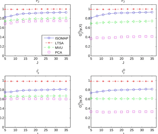
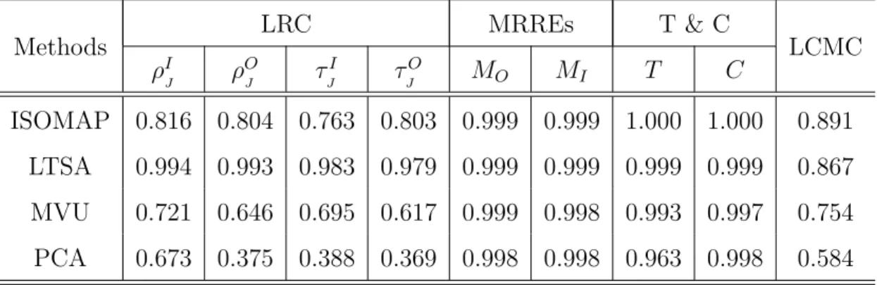
2.1 Assessing ISOMAP, LTSA, MVU, PCA in Swiss Roll data (J = 6) . . . 56 2.2 Assessing ISOMAP, LTSA, MVU, PCA in S-curve data (J = 6) . . . 56 2.3 Assessing ISOMAP, LTSA, MVU, PCA in sculpture face image data (J = 6) 59

(11)

List of Figures

2.1 Illustration of AR and LCMC. . . 38

2.2 Illustration of output normalized methods. . . 40

2.3 Failure of the naive measure. . . 43

2.4 The Swiss roll and the S-curve . . . 49

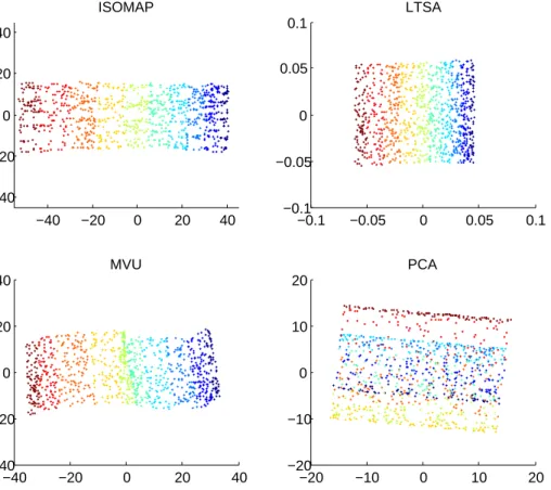
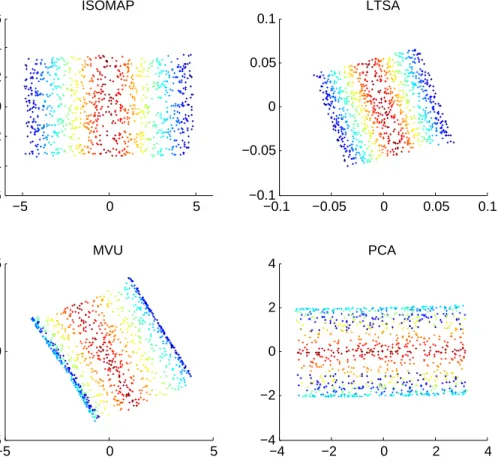
2.5 Two-dimensional output configurations of different methods for the Swiss roll 50 2.6 Low-dimensional configurations of different methods for S-curve . . . 51

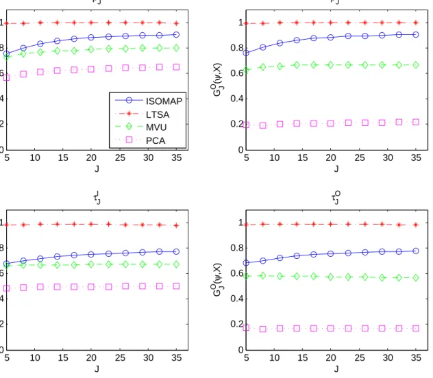
2.7 Local Spearman correlation as functions of J in the Swiss roll . . . 52

2.8 Local Spearman correlation as functions of J in the S-curve . . . 53

2.9 Histogram of ρO J (J = 6) in the Swiss roll . . . 54

2.10 Histogram of ρI J (J = 6) in the Swiss roll . . . 55

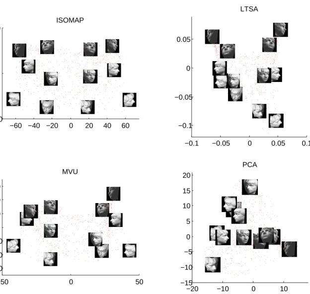
2.11 2-dimensional configurations from ISOMAP, LTSA, and PCA for sculpture face image . . . 57

2.12 Local rank correlation as functions ofJ in sculpture face image . . . 58

(12)

2.14 Low-dimensional configurations with different values ofK . . . 60

2.15 Local rank correlation as a function of K (J = 6) . . . 61

2.16 Local rank correlation as a function of dimensionality q (J = 6) . . . 63

3.1 Visualizing the influence function of PCA . . . 80

3.2 The empirical influence function of Kernel PCA with a polynomial kernel . 81 3.3 The empirical influence function of LLE and ISOMAP . . . 82

3.4 Detecting influential observations. (a) EIF(j)with sample estimates of eigen-values and eigenvectors. (b) EIF(j)with true values of eigenvalues and eigen-vectors. . . 83

3.5 Sample influence functions of (a) PCA, (b) ROBPCA, (c) LLE, and (d) ISOMAP. . . 87

3.6 Sample influence functions of ISOMAP . . . 89

4.1 PCA from the viewpoint of bagging . . . 96

4.2 Effect of subsample size m (K = 50) . . . 103

4.3 Effect of number of subsample K (m= 5) . . . 104

4.4 Monotonic transformation of weights w_k. . . 108

4.5 Histogram of weights w_k with and without transformation (= 0.2). . . 109

4.6 Effect of transformation on the weight function. . . 109

4.7 Histogram of estimated subspace dimension q_k . . . 115

(13)

4.9 Simulation case (i). . . 118

4.10 Simulation case (ii). . . 119

4.11 Background modeling in escalator surveillance video data by Performance-Weighted Bagging PCA (algorithm 1). . . 121

4.12 Background modeling in escalator surveillance video data by Performance-Weighted Bagging PCA (algorithm 2) and principal component pursuit. . . 122

4.13 Player detection in basketball video data by Performance-Weighted Bagging PCA (algorithm 1). . . 124

4.14 Player detection in basketball video data by Performance-Weighted Bagging PCA (algorithm 2) and principal component pursuit. . . 125

4.15 Three frames from the original video (upper row), and three random noise images (lower row). . . 126

4.16 Foreground objects detection with clean data. . . 127

(14)

List of Abbreviations

AR Agreement rate metric

Bagging Bootstrap aggregating

BP Breakdown point

EIF Empirical influence function

IF Influence function

KPCA Kernel Principal component analysis

LCMC Local continuity meta criterion

LLE Local linear embedding

LRC Local rank correlation

LTSA Local tangent space alignment

MDS Multidimensional scaling

(15)

MSD Mean square distance

MVU Maximum variance unfolding

PCA Principal component analysis

PCP Principal component pursuit

PP Projection pursuit

RV Residual variance

SC Sensitivity curve

SIF Sample influence function

SVD Singular value decomposition

(16)

Chapter 1

Introduction and Overview

1.1

Review of robustness

Robust statistics are a class of statistical procedures which are created to deal with an in-stability problem of the optimal procedures of classical methods. The use of term “robust-ness” can be traced back to George Box [1953], who discussed in his paper the sensitivity to non-normality of some statistical tests. Subsequently, John Tukey [1960; 1962], Peter Huber [1964; 1965; 1981], and Frank Hampel [1968] gave respective contributions toward the foundations of robust statistics. Since then it has been systematically investigated and developed by many other researchers. Nowadays robust statistics are an important alternative to the classical approaches. To better understand this concept, three questions must be answered: What is robustness? Why use robust procedures? And how does one measure robustness?

(17)

1.1.1

What is robustness and why it is needed

All statistical models and methods include assumptions on the underlying distribution, such as normality, linearity, independence, etc. These assumptions are either for mathe-matical convenience or based on previous experience, and an inference one makes relies not only on the observed data, but also on these assumptions. Most of traditional statistical methods are optimal only when their assumptions are satisfied.

However, it is generally understood that these assumptions are at most an approxima-tion to reality. In practice, the appearance of outlying data caused by either gross error (large errors in measurement, see Dixon [1953]; Grubbs [1969]) or flaws in model assump-tions often occur. Thus, besides considering criteria of optimality, it is natural for one to expect that a statistical procedure is stable in the sense that a small departure from the model assumptions or a small proportion of outlying data will only cause a small error in the final conclusion, so that the procedure can still provide a good result.

Unfortunately, statistical procedures are not always stable. In the 19th and 20th cen-turies, statisticians (such as S. Newcomb, K. Pearson, H. Jeffreys, and E. S. Pearson) were aware of the instability of some traditional methods, and in recent decades, studies point to the fact that even some commonly used statistical procedures are excessively sensitive to seemingly minor deviations from model assumptions. Sometimes these deviations will even cause the breakdown of the procedure (Hampel [2001]).

In many location parameter estimation problems, the sample mean is a common choice. The following example illustrates the performance of the sample mean when model assump-tions are violated.

Example 1.1. Robustness of sample mean: Suppose we have a sample of observationsxi,

(18)

traditional choice is the sample mean, which is unbiased and attains the smallest variance at the assumed model. However, if the normality assumption is not exactly correct, the performance of the sample mean might not be good (as measured by the variance and bias).

Let the observations come from the following distribution:

Xi ∼        N(µ, σ2₎ _{with probability 1}₋ f(x) with probability ,

where f(x) is some non-Normal distribution with mean θ and variance τ2. Then it is easy to calculate that Bias(X) =(θ−µ), Var(X) = (1−)σ 2 n + τ2 n + (1−)(θ−µ)2 n .

Even if is very small (i.e. Xi is approximately Normal), the variance and bias of X

could become arbitrarily large or even infinite (e.g. when f(x) is the Cauchy pdf).

As illustrated in the above example, the optimal estimator (in the sense of efficiency) for the Normal location parameter, will provide a poor result even under a slightly con-taminated model.

This fact motivates statisticians to create the concept of “robustness” to study the ef-fect of wrong assumptions on a given statistical method. Robustness is considered to be a property of a statistical procedure, which describes its behavior under violations of the

(19)

model assumptions. As stated by Huber [1981], “robustness signifies the insensitivity to small deviations from assumptions”. The effect of wrong assumptions is not limited to the parameter estimation problem (Example 1.1), the importance of studying robustness of statistical procedures is recognized by statisticians in hypothesis tests (Gastwirth and Ru-bin [1971]; He et al. [1990]; He [1991]), regression (Rousseeuw [1984]; Ruppert and Carroll [1971]), mixed models (Welsh and Richardson [1997]), and almost all areas of statistical research. Furthermore, many robust procedures were proposed as reliable alternatives to traditional procedures, aiming to provide reasonable results when the model assumptions are not exactly satisfied.

Alternatively, to avoid the study of robustness, it might be possible to build up a diagnostics system to test the model assumptions and clean the data before applying the traditional methods. Based on this idea, many detection techniques were developed (e.g. outlier rejection, normality tests. See Hawkins [1980]; Hodge and Austin [2004]), but unfortunately these rules are not enough to replace the role of robustness for several reasons.

First of all, traditional outlier detection methods have difficulties in dealing with mask-ing and swamping (See Fieller [1976]; Barnett and Lewis [1984]). It is discussed by some researchers that even the best rejection rules do not achieve the expectation of completely identifying the violation of model assumptions (Hampel et al. [1986]; Hampel [1974]). Sec-ondly, the criteria for detection and rejection are usually subjective so these rules often suffer from false rejection and false retention error, which will cause a significant loss of ef-ficiency (Hampel [1985]). Thirdly, lots of diagnostics approaches are closely related or even based on robust methods (Barnett and Lewis [1984]; Gather and Becker [1997]). Moreover, when the diagnostics show that some assumptions do not hold (e.g. independence), there does not always exist a well-established alternative approach to deal with the violation.

(20)

Thus, robustness provides a safeguard against the situation when the model is not exactly true but this fact is difficult to be detected.

1.1.2

Contamination models and outliers

The uncertainty in the model assumption results in the discordant observation in the sample, usually referred as “outlier” (Beckman and Cook [1983]). An outlier is defined as “one that appears to deviate markedly from other members of the sample in which it occurs” (Grubbs [1969]). There are two main reasons for the appearance of outliers.

• Case I. The presence of gross error. In this case, one believes that the majority of the observations comes from the assumed model, while the remaining observations are from outside the population being examined. These contaminated observations are considered to be bad for the inference because they are non-informative for the assumed model and may corrupt the clean data.

• Case II. The model misspecification. In this case, the assumed model oversimplifies or provides an incorrect description of the data. For example, normality is a key assumption for many traditional methods in regression, analysis of variance and multivariate analysis. However this assumption is invalidated if the error distribution has heavy tails (Newcomb [1886]). Mistakenly assuming the normality might have a serious effect on the conclusion.

These two cases lead to two different types of robustness: firstly the robustness against the gross error, and secondly the robustness against the model misspecification (Maronna et al. [2006]). They share the term robustness but represent different philosophies. The first one is based on the faith that the model is close enough to the underlying truth, and

(21)

focuses on the effect of suspicious points on the result, whereas the second one believes the cleanliness of the data, and tries to check the adequacy of model assumptions.

Thus, although outliers can occur due to both gross errors and model misspecification, we will only use the term “outlier” in the first case (i.e. the gross error case) to avoid confusion.

A commonly used tool to formalize the uncertainty of the model assumptions in the distributional setup is the -contamination model (introduced by Tukey [1962]; Huber [1964]). Let Xi (i = 1. . . n) be independent random variables with common distribution

H such that

H(x) = (1−)·F(x) +·G(x) (1.1) where Fis the assumed distribution in the model,G is a unknown contaminating distribu-tion (possibly with some restricdistribu-tions), and 0 ≤ <1 is a real number. The contamination level of model (1.1) is usually measured by , which measures the difference between as-sumed model F and true model H. Example 1.1 is an application of the-contamination model. In addition toin equation (1.1), one can also use other distance functions defined on distribution space to measure the difference between the assumed model and the true model (See V´ıˇsek [1997]; Huber [1981]).

Instead of considering contamination in the distributional sense, we can also define contamination models in a finite sample setup (Donoho and Huber [1983]). Let xn =

(x1, . . . , xn)0 be a column vector representing a fixed sample of sizen, wherex0 denotes the

transpose of the matrix or vectorx. There are two ways to model the sample contamina-tion:

(22)

arbitrary values ω1, . . . , ωm. Let x(n,m) denote the contaminated sample, and the

contamination level is =m/n.

(ii) -corruption: we adjoin marbitrary additional pointsωωωm = (ω1, . . . , ωm)0 to the

orig-inal xn. Letxn,m =xn∪ωωωmdenote the contaminated sample, and the contamination

level is =m/(n+m).

Note that although outliers can occur due to both gross errors and model misspecifica-tion, we will only use the term “outlier” in the first case, i.e. the gross error case.

1.1.3

Measures of robustness

Considering both optimality and robustness, as argued by Huber [1981] and Hampel et al. [1986], an ideal statistical procedure should satisfy three criteria:

• It should have a high (optimal or nearly optimal) efficiency when the model assump-tions hold.

• It should be resistant to slight contamination to the model, i.e. the loss of efficiency due to the variation of assumptions should be as low as possible.

• A small violation of model assumptions will not completely spoil the procedure.

To investigate the second and third points in detail, many different types of measures have been proposed to monitor the decrease of performance of a statistical method due to the contamination. We now discuss these criteria.

(23)

Influence function

A widely used and well accepted robust measure is the influence function (IF). This concept was introduced by Hampel in his Ph.D. thesis (Hampel [1968]), and further developed in 1974 (Hampel [1975]). In the paper Hampel considers a statistical estimator as a functional

T mapping from the space of probability distributions F to a parameter space of interest,

T :F →_R.

The influence function is defined as the Gˆateaux derivative of the functional T, at the assumed distribution F ∈ F and a certain point x ∈ _Rd _{based on one-step Taylor}

expansions ofT. It is defined by IF(x; T, F) = lim ↓0 T((1−)F+δx)−T(F) = ∂ ∂T((1−)F+δx)|↓0, (1.2)

whereδx is the point-mass at x.

The influence function is a local concept since it measures quantitatively the change of T according to the point-mass contamination at a certain x. A procedure T is more sensitive (than others) to the contaminationδx if it has a larger (in absolute sense) value

of the influence function atx. Thus, for the sake of robustness, the influence function of a procedure is desired to be bounded. For instance, the classical mean functional

T(F) =

Z xdF,

(24)

Hampel also proposed a way to find estimators with optimal efficiency given an upper bound on the influence function (Hampel et al. [1986]). General discussion of influence functions can be found in Serfling [1980], Huber [1981] and Hampel [1974]; Hampel et al. [1986].

Several different types of the finite sample influence function have been developed for use in practice. A direct sample version of influence function, usually called the empirical influence function(EIF), is defined similar to the influence function, where the probability distributionF is replaced with the empirical distributionFb_nof the sample. Another

finite-sample version is defined in Tukey [1970], called the sensitivity curve, or sometimes also called the empirical influence function or sample influence function. One adds a virtual observation xto the sample X ={x₁, . . . , xn}and assesses its influence on the estimate T

by

SC(x; T, X) = (n+ 1){T(x₁, . . . , xn, x)−T(x1, . . . , xn)} .

Both the empirical influence function and the sensitivity curve are to evaluate the effect on an estimate of perturbing an observation at a finite sample. Mallow [1975] discussed different definitions of the sensitivity curve under different types of contamination when a new observation is added, the i-th observation is replaced, or deleted. The sensitivity curve is essentially equivalent to the empirical influence function, and it converges to the influence function asn→ ∞ (Hampel et al. [1986]; Maronna et al. [2006]).

Breakdown point

The influence function is a useful tool to assess the robustness of a statistical procedure. However, as pointed out in Lindsay [1994], considering only local measures might poorly assess the robustness of some types of estimators. Thus, besides the information about

(25)

the local behavior of a procedure near the assumed model, one may also want to investi-gate a global measure which indicates how much assumptions may be violated before the statistical procedure becomes invalid.

The breakdown point (or breakdown value) is a global robustness measure, concerning the extreme situation when the procedure is ruined (called “breakdown”). The concept was first proposed by Hodges [1967] (as “the tolerance of extreme value”) in the location estimation problem. Hampel provided the formal definition of asymptotic breakdown point (Hampel [1968, 1971, 2005]). Donoho [1982] and Donoho and Huber [1983] proposed the finite-sample version breakdown point, and had a general discussion on the application of breakdown points. The intuition beneath the breakdown point is to measure the minimum proportion of contamination in the sample (or in model assumption) that can cause the breakdown of the procedure.

In the framework of Huber’s functional analytic approach to robustness, breakdown is related to the boundedness of statistical functionals. Donoho and Huber [1983] mathemat-ically formalized the “breakdown” phenomenon as that for which the functional is carried beyond the bounds of the parameter space (if it is bounded).

Consider a measurable sample space (Ω,B(Ω)) where Ω is the sample space and B(Ω) is the Borelσ-algebra. Let F be the family of all nondegenerate probability measures (or distributions) on (Ω,B(Ω)), with a metric d on F such that

sup

F,H∈F

d(F,H) = 1 (1.3)

Let T : FT → Θ be a statistical functional, mapping a subspace FT ⊆ F into some

(26)

sup

θ1,θ2∈Θ

D(θ1, θ2) =∞ (1.4)

Definition 1.1. Asymptotic breakdown point: For a given functional T, and appropriate metrics D and d on Θ and F respectively that satisfying (1.3) and (1.4), the asymptotic breakdown point ofT at a given distributionF∈ FT is defined by

∗(T,F) = inf ( >0 : sup d(F,H)< D(T(F), T(H)) = ∞ ) (1.5)

Example 1.2. Asymptotic breakdown point of mean: LetT be the expectation functional

TE(F) =

Z

Ω

xdF(x).

Choose d to be the Kolmogorov-metric

d(F,H) = sup

x∈Ω

|F(x)−H(x)|,

and D to be the Euclidean metric on Θ (Θ = _R). Then it can be verified (Davies and Gather [2007]) that

∗(TE,F) = 0,

for anyF ∈ FT, where FT ={F:TE(F)<∞}.

The asymptotic breakdown point is defined on the probability distribution of the as-sumed model. Similarly, the finite sample version of breakdown point can be defined on the empirical distribution of the sample.

Definition 1.2. Finite sample breakdown point: Given an appropriate metric D, and a sample xn = (x1, . . . , xn) of size n, the empirical distribution of xn is denoted by Fb_n =

(27)

1

n

Pn

i=1δxi, where δxi is the Dirac measure. The finite sample breakdown point of T at the

samplexn (or at empirical distribution Fb_n), is defined by

fsbp(T,xn) = 1 n min ( m∈ {1, . . . , n}: sup x(n,m) D(T(Fb_n), T(Qb₍_n,m₎)) =∞ ) (1.6)

wherex(n,m) is the samplexn with m points replaced by arbitrary value, andQb₍_n,m₎∈ F_T

is the empirical distribution ofxn,m.

Example 1.3. Finite sample breakdown point of median: Given a samplexn = (x1, . . . , xn)

of size n (assume n is odd for convenience), and let T be the sample median functional

Tmed(xn) = x((n+1)/2), and Θ, D be the same as in example 1.2. Then it can be verified

(Davies and Gather [2007]) that

fsbp(Tmed,xn) =

n+ 1 2n

In above definitions, the usual choice of metric D is the Euclidean metric, d is Kol-mogorov metric or Prohorov-metric (Huber [1981]), and the statistical functional T rep-resents a particular estimator. Davies and Gather discuss the choice of metric D and d

(Davies and Gather [2007]), and also emphasize the importance of affine groups structure (Davies and Gather [2005]) in comparing statistical functionals in terms of breakdown points.

Definition 1.1 and 1.2 are well accepted because of their simplicity and intuition. They have been applied in location and scale parameter estimation and linear regression prob-lem (Yohai [1987]; Donoho and Gasko [1992]; Ellis and Morgenthaler [1992]; Davies [1993]; M¨uller and Uhlig [2001]). The concept of breakdown point is also generalized to cope with other statistical problems including testing (He [1991]; He et al. [1990]), multivariate anal-ysis (Rousseeuw [1985]; Gordaliza [1991]; Lopuha¨a [1992]; He and Fung [2000]), directional

(28)

data (He and Simpson [1992]), nonlinear regression (Stromberg and Ruppert [1992]), and time series (Lucas [1997]; Mendes [2000]; Ma and Genton [2000]; Genton [2003]).

However, the standard definition has some limitations (Genton and Lucas [2003]), and attempts have been made to obtain a more general definition of breakdown points by formalizing the concept of “breakdown” from different perspectives (Sakata and White [1995]; He and Simpson [1993]; Genton and Lucas [2003]).

Among the affine equivariant estimators, it is possible to calculate the upper bound of the breakdown point in many statistical problems (Davies and Gather [2007]), and estimators with highest possible breakdown points are develeped. However, to fully under-stand the robustness of a statistical procedure requires the combination of different types of robustness measures. Simply pursuing the highest possible breakdown point may be misguided (see Huber and Ronchetti [2011]; He and Portnoy [2000]).

Other robustness measures

The influence function and breakdown point consider the extreme situations of contami-nation. The influence function considers infinitesimal values of and the breakdown point seeks for the smallest contamination level? _{under which a procedure becomes invalid.}

Hu-ber [1964] proposed another measure which allows one to study the behavior of a procedure under a fixed contamination level (before breakdown). He introduced several distance-based neighborhoods to model the deviation from assumptions, and further considered the worst asymptotic performance (in the sense of variance or bias) of a procedure under a certain contamination level. These measures are known as minimax asymptotic variance (MV) and minimax bias (MB), or sometimes referred as maximum asymptotic variance and maximum bias (Huber [1964, 1981]). Using the contamination model (1.1), the MB

(29)

and MV of the statistical functional T at a distribution F∈ F are defined as MB(F, T, ) = sup G∈F |T((1−)F+G)−θ| (1.7) MV(F, T, ) = sup G∈G Var [T ((1−)F+G)] (1.8) Based on this idea, Huber developed a class of robust procedures whose worst asymp-totic performance is minimized (called the minimax approach). It has been shown that these approaches have some good finite sample properties (see Andrews et al. [1972]). Other similar measures based on the same idea include the bias curve (Rousseeuw and Croux [1994]), contamination sensitivity and gross-error sensitivity (Hampel [1968]).

Besides these quantitative measures, Hampel [1971] also introduced the concept of qualitative robustness which is closely related to the influence function and the breakdown point. Since Hampel, further theoretical development has been made by Cuevas [1988], and applications can be found in Lambert [1982]; Rieder [1982]; Boente et al. [1987]; Papantoni-Kazakos [1984].

1.2

Introduction to dimensionality reduction

With the development of data collection and storage capabilities, researchers across a wide variety of fields are facing larger and larger datasets with increasing dimensionality, such as images, videos, fingerprints, text documents, etc. Higher dimensionality brings challenges together with benefits. More variables provide more information for inference, but at the same time, the size of data needed for a reliable result increases exponentially with the dimensionality (See Bellman [1961]; Donoho [2000]), therefore traditional statistical methods have difficulties to cope with the explosive growth of dimensionality.

(30)

To solve this, dimensionality reduction methods have been developed and applied as pre-processing tools to deal with such high-dimensional datasets. The foundation of di-mensionality reduction is the belief that there exists some underlying (unknown) geometric structure in the observed high-dimensional data which allows us to use a lower dimensional representation to characterize the data without losing this structure. Thus, the purpose of the dimensionality reduction methods is to reveal this structure.

Revealing the low-dimensional representation not only improves the efficiency of com-putation, but also enhances the understanding of the nature of the data. Over the last few decades, many dimensionality reduction algorithms have been proposed. Summaries and surveys can be found in many books and papers (Carreira-Perpinan [1997]; Friedman et al. [2009]; Fodor [2002]) and new ideas are still being contributed to the area. To better illustrate these ideas, we need to first introduce some geometric concepts and notations.

1.2.1

Topology and manifolds

We assume the readers have enough background knowledge about topology, topological space and geometry, and are familiar with basic concepts (such asopen sets,neighborhood,

C∞ maps, connected spaces, homeomorphism, tangent spaces, etc. Mathematical details can be found in Kelley [1955]; Armstrong [1979]; Lee [2000, 2003]) .

Manifold

Suppose Mis a topological space. We say Mis a topological d-manifold if it satisfies the following conditions:

• Mis aHausdorff space: For allp, q ∈ M, there exist disjoint open subsetsU, V ⊂ M such that p∈U and q∈V.

(31)

• M issecond countable: There exists a countable basis for the topology ofM.

• Mislocally Euclidean of dimension d: For allp∈ M, there exist open setsU ⊂ M,

e

U ⊂_Rd _{such that} _p_∈_U _{and there exists a homeomorphism} _φ _:_U _→_U_e_.

The dimensionality ofMisd, and the manifold is denoted as Md _{in this paper if we want}

to emphasize its dimensionality.

Achartfor a topological space Mis a homeomorphism φfrom an open subset U ⊂ M to an open subset in Euclidean space, it is usually denoted as (U, φ). Based on this notion, we can define two important concepts:

• Atlas: An atlas Afor a topological space Mis a collection of chartsA={(Uα, φα)}

on Msuch that S

Uα =M.

• Transition maps: Provide two charts (Uα, φα) and (Uβ, φβ) for a topological space

M such that Uα∩Uβ 6= ∅, the transition mapτα,β : φα(Uα∩Uβ) → φβ(Uα∩Uβ) is

defined as:

τα,β =φβ◦φ−α1.

A topological manifoldMis said to be a differentiable manifold if it is equipped with an atlasA={(Uα, φα)} such that for all φα, φβ ∈A, the transition mapτα,β is differentiable.

An atlas satisfies such conditions is called a differentiable structure on M. A simple example of differentiable manifold is the Euclidean space_Rd_.

Embedding and embedded submanifolds

Given a differentiable manifold ND_{, a} _d_-submanifold _Md _{⊂ N}D ₍₀ _{< d} _≤ _D_{) is}

(32)

(U ⊂ N, φ : U → _RD_{) such that} _p _∈ _U_, _φ _{is a diffeomorphism, and} _φ_{(M ∩}_U_{) is a} _d_-flat

in _RD_.

In dimensionality reduction problems, manifolds can be characterized as embedded submanifolds of Euclidean space by Whitney embedding theorem (Whitney [1936]). A simple example is that a m-sphereSm _{is an embedded submanifold of}

Rm+1. In this paper,

we use the term “manifold” to refer the (differentiable) embedded submanifold of some Euclidean space unless specified otherwise, i.e. Mmeans Md _⊂

RD (for somed ≤D).

Suppose M and N are two differentiable manifolds, and f : M → N is a C∞ map. The mapping f is said to be an embedding if it satisfies:

• f is an immersion: the derivative off is injective at every point p∈ M.

• f is a homeomorphism onto its image f(M)⊂ N in the subspace topology.

The imagef(M) is called an immersed submanifold of N, andMis said to be embedded inN by the mapping f.

Riemannian manifold and geodesics

Consider a pointpon a differentiable manifoldM. All vectors that are tangent toMat the pointpwill form a vector spaceTp(M) called tangent space atp. Suppose that for every

point pon M, the tangent space has an inner-product gp =h·,·i :Tp(M)×Tp(M)→R.

The collection of inner-products g = {gp|p∈ M} is called a Riemannian metric on M,

and the manifold equipped with a Riemannian metric is called a Riemannian manifold, denoted as (M, g).

Given a manifold M, and two points p, q ∈ M, a smooth curve on M from p to q

is defined as a continuous map ζ : I → M ⊂ _RD_{, where} _I _{= [}_{a, b}_] _⊂

(33)

ζ(b) = q. The smooth curve joins points p and q are not unique, let Cpq be the collection

of all such curves. With the metric g defined on M, we can calculate the length of any smooth curve on the manifold:

L(ζ) =

Z b

a

q

g(ζ0₍_t₎_{, ζ}0₍_t₎₎_dt, and the distance betweenp and q on Mis defined as

dM(p, q) = inf

ζ∈Cpq L(ζ).

The distance dM(p, q) is called the geodesic distance on the manifold M. If M is a Euclidean space, the geodesic distance would be the Euclidean distance.

1.2.2

Problem setup

In dimensionality reduction, we assume that the observed data in high-dimensional space lie on (or near) an embedded submanifold with lower dimensionality. With this fundamental assumption, it is possible to represent the high-dimensional data in a lower-dimensional space. Formally, we state the problem as following: suppose that there aren data points in aq-dimensional space_Rq, denoted by a set of column vectors{y₁, . . . ,yn}, or together by an

n×qmatrixYwithj-th row being the transpose of thej-th data pointy0_j. Further assume

yj are mapped into a higher-dimensional space Rp by an unknown smooth embedding

ϕ:_Rq _{→ M}q _⊂

Rp (p > q) possibly with noise:

xj =ϕ(yj) +j, (1.9)

where j ∈Rp, j = 1, . . . , n is the noise with mean 0. We refer “case j” as the index of the

(34)

We only observe {x1, . . . ,xn} in Rp, together denoted by an n×p matrix X. We say

{x1, . . . ,xn}lie on (or near) the manifoldMwithintrinsic dimensionality q, or we say the

intrinsic dimensionality of Xis q. The purpose of dimensionality reduction algorithms are essentially trying to reconstruct the inverse mappingψ =ϕ−1, and to recoverybyyb =ψb(x)

(sometimes we only recoveryb with implicitψb). We denote a given dimensionality reduction

method as a mappingψ :_Rp _→

Rq in the rest part of the thesis. In many methods, ψ is a

function of the entire observed dataset, so we also write the low-dimensional configuration

Y asY =ψ(X) for convenience.

This type of dimensionality reduction can be also viewed as learning the structure of embedded submanifold Mq_{, so it is also called manifold-learning. In this thesis, we shall}

restrict our attention to manifold-learning. Different algorithms have different assumptions onψ. According to these assumptions we can roughly classify the dimensionality reduction algorithms into two major types: linear methods and non-linear methods.

1.2.3

Linear methods

In general, linear dimensionality reduction methods assume that the embedded subspace is a linear subspace, and look for a linear projection to recover y:

b

y=ψb(x) =W0x(or directly Yc=X W) (1.10)

where W is a p×q projection matrix. Choosing W due to different criteria determines different algorithms.

Principal component analysis (PCA) is a popular and well-known linear method. It was introduced by K. Pearson [1901], and also known in different fields of application as singular

(35)

value decomposition (SVD), empirical orthogonal functions (EOF), the Karhunen-Lo`eve transform, and the Hotelling transform.

In essence, PCA seeks a linear subspace formed by a set of orthogonal vectors called “principal components” in such a way that the variability of the data is kept as much as possible in the subspace. Given observed data pointsXand assuming zero empirical mean, the orthogonal basis (principal components){wj} are a set of p×1 unit vectors that are

obtained by w₁ = arg max kwk=1 {kXwk}, and for 2≤k ≤p w_k = arg maxnkXwk kwk= 1, w⊥wj,∀1≤j ≤k o ,

where kwk is the Euclidean norm of the vector w. In practice, the principal components

n

wj

o

are calculated by the eigendecomposition of the empirical covariance matrix of the observed data (assuming that the data are centered on the origin, i.e. Pn

j xj = 0): C= 1 n n X j=1 xjxj0 = 1 nX 0_X_.

The k-th principal component is the eigenvector ofCcorresponding to itsk-th largest eigenvalue. If the essential assumption that the data actually lie on or near aq-dimensional linear subspace holds (assuming q is known here), we would find that the firstq principal components carry most of the variability and then we can disregard the remaining principal components, and project the data onto a low-dimensional space spanned by the orthogonal basis W= (w1,w2,· · · ,wq).

(36)

PCA can be also solved in a dual form. The singular value decomposition (SVD) of X

gives

X=UΛΛΛW0,

where columns of Uare topqeigenvectors of X X0, columns ofWare topq eigenvectors of

X0X, and the diagonal matrix ΛΛΛ contains the square roots of eigenvalues of bothX0X and

X X0. Note that there exists a one-to-one correspondence between Uand W. Therefore, obtaining Un×q and ΛΛΛq×q from the eigendecomposition of X X0 will also lead to the

low-dimensional representation of PCA,

W=X0UΛΛΛ−1

c

Y=X W=UΛΛΛ.

This dual form is typically helpful when the dimensionality p of the input data X is very large (pn).

Multidimensional scaling (MDS) is another classical linear technique which encompasses a collection of methods (Cox and Cox [1994]). Whereas PCA tries to preserve the vari-ability of the data in low-dimensional space, MDS focuses on the pairwise relations (called distance, proximity or dissimilarity) and attempts to provide a geometrical representation of these relations.

MDS takes a pairwise proximity matrix D = [dij]n×n as input, where dij is a measure

of closeness between objects xi and xj, and is trying to construct a configuration by

mini-mizing some loss function. There are many versions of MDS algorithm depending on the choice of dij and loss function, two major classes are metric and non-metric MDS.

Metric MDS chooses dij to be a metric of the original space (not necessarily Euclidean

(37)

c Y= arg min Y X X 1≤i<j≤n dij −db_ij 2 ,

wheredb_ij =ky_i−y_jk2, andk·kis the Euclidean norm. Choosingd_ij as Euclidean distance

in_Rp will obtain the same result as PCA. In general, MDS can be solved by eigendecom-position of the matrix D, defined by the squared pairwise metric.

In contrast, non-metric MDS tries to preserve the ordinal property of the data rather than the proximity, and the loss function called Stress (Cox and Cox [1994]) is applied.

Stress = v u u u u u t P P 1≤i<j≤n f(dij)−dˆij 2 P P 1≤i<j≤n ˆ d2 ij ,

where f(dij) is a monotonic transformation. An iterative algorithm was proposed by R.

Shepard [1962] and then refined by J. Kruskal [1964] to minimize Stress and obtain the solution of non-metric MDS.

PCA and MDS are both widely used linear algorithms. However their usefulness is limited by the global linearity of the submanifold. Other linear methods such as factor analysis, projection pursuit, independent component analysis, also share this limitation and cannot provide a satisfactory result if the underlying submanifold does not have the global linearity.

1.2.4

Nonlinear methods

Motivated by the inability of linear methods to capture the nonlinear structure, many nonlinear methods have been developed, including ISOMAP (Tenenbaum et al. [2000]), Local Linear Embedding (Roweis and Saul [2000]), Laplacian Eigenmap (Belkin and Niyogi

(38)

[2001, 2003]), Local Tangent Space Alignment (Zhang and Zha [2005]), Self-organizing map (Kohonen [1982, 1990]), Kernel PCA (Sch¨olkopf et al. [1998]), Maximum Variance Unfolding (Weinberger and Saul [2006b,a]), Diffusion Maps (Nadler et al. [2005]), and many different versions of nonlinear PCA (Gnandesikan and Wilk [1969]; Hastie and Steutzle [1989]; Kramer [1991]).

Comparing to the linear methods, the nonlinear methods relax the global linearity assumption about the submanifold, and instead adopt two additional assumptions:

• The embedding ϕ : _Rq _{→ M} _{is a} _{local isometry}_{: for each} _z _∈

Rq, there exists a

neighborhood U of z such that

dq(y1,y2) = dM(ϕ(y1), ϕ(y2)), y1,y2 ∈U

where dq is the Euclidean distance in _Rq, and dM is the geodesic distance on M. • The observed data points are dense enough on the manifold: for eachx∈ {xj}, there

exists a set Nx of neighboring points such that

dM(x,xi)≈dp(x,xi), xi ∈Nx,

where dp is the Euclidean distance in _Rp. The set Nx is called the neighborhood of x.

Given above two assumptions, and equation (1.9), we can have dq(yi,yj)≈ dp(xi,xj)

if xi and xj are neighboring points. Most of the nonlinear methods are considered to be

local methods because they focus on the local geometry of the submanifold, and try to recover {yj} by preserving the neighborhood relationship. These methods usually consist

(39)

• Step 1: Identify the neighborhood Nx for each data point. Usual ways of identifying

the neighborhoods are

K-nearest neighborsNx,K (measured by Euclidean distance)

-ball: Nx,={xi ∈ {xj} |dp(x,xi)≤}

where k and are tuning parameters (usually called neighborhood size). Note that in general, xi ∈Nxj does not necessarily imply xj ∈Nxi.

• Step 2: Characterize the neighborhood relationship (the relationship is formalized differently in different methods).

• Step 3: Construct the low-dimensional configuration that optimally preserve the specified neighborhood relationship.

A typical local method is Local Linear Embedding (LLE). After assigning the neigh-borhood to each point, LLE characterizes the neighneigh-borhood relationship by a set of linear coefficients that reconstruct each data point from its neighbors. The linear coefficients {wij} are obtained by minimizing the reconstruction error:

c W = arg min W n X i  x_i− n X j wijxj   2 ,

wherewij satisfieswij = 0 ifxj ∈/ Nxi, and

Pn

j wij = 1.

Assuming that the coefficients Wc are invariant to the mapping ϕ, the same weights

{wbij} that reconstruct the data point xi should also be able to reconstruct the

corre-sponding point yi in the embedding space. Thus, the low-dimensional representationcY is

constructed by minimizing the embedding cost function:

c Y= arg min Y n X i  y_i− n X j b wijyj   2 ,

(40)

The properties and limitations of LLE and the complexity of the algorithm are discussed in Roweis and Saul [2000].

Besides the local methods, there is another class of nonlinear methods which consider the global geometry of the submanifold (usually referred as global methods). A typical one in this class is ISOMAP.

ISOMAP considers the global geometry by assuming the mappingϕis an isometry, i.e.

dq(y1,y2) =dM(ϕ(y1), ϕ(y2)), y1,y2 ∈Rq,

ISOMAP can be viewed as a generalization of metric MDS because it carries the idea of MDS, and tries to preserve the pairwise geodesic distances (instead of Euclidean distances).

The algorithm also starts with identifying the neighborhood for each point. This results in a weighted neighborhood graphG = (V,E), where the set of vertices V ={xj} are the

observed data, and the set of edgesE ={eij}indicate the connection between two points. If

xi andxj is assigned as neighboring points (i.e. at least one of them is in the neighborhood

of the other), the edge eij has a weight wij =dp(xi,xj).

The next step is to approximate the pairwise geodesic distance based on the graph G. A path P in the graph is defined as a sequence of vertices P = (v1, . . . , vm) such that for

all 1≤i≤m−1, vi and vi+1 are neighboring points. The length of the pathP is defined

as dG(P) = m−1 X i=1 wi,i+1.

Non-neighboring vertices xv and xu are connected by any pathPuv = (v1, . . . , vm) such

thatv1 =xv andvm =xu. The graph distance (also called shortest path distance) between

xv and xu is defined as

dG_uv = min

Puv

(41)

The graph distance can be efficiently calculated by Floyd’s algorithm (Floyd [1962]) or Dijkstra’s algorithm (Dijkstra [1959]). Then the geodesic distances are approximated by:

b dM_ij ≈        dp(xi,xj) if xi,xj are neighbors,

dG_ij if xi,xj are not neighbors.

The final step is to apply metric MDS to reconstruct the low-dimensional configuration

c

Y, with the input being the pairwise geodesic distance matrix DG =hdbM_ij i

n×n.

It has been shown that with some regularity conditions, the graph distance converges to the true geodesic distance as the sample size n → ∞ (Bernstein et al. [2002]). It worth mentioning that ISOMAP additionally assumes convexity on the submanifold M. This assumption is important for approximating the geodesic distances, but it appears to be too restrictive in many instances (Donoho and Grimes [2003]). The performance of ISOMAP is discussed in Donoho and Grimes [2002b], and several modified versions have been developed in order to relax the model assumptions (Donoho and Grimes [2002a]; Silva and Tenenbaum [2002]).

1.2.5

Kernel PCA and a unified framework

Kernel PCA (Sch¨olkopf et al. [1997]) is another type of nonlinear dimensionality reduction method. The Kernel PCA performs principal component analysis in a feature space which is related to the original input space by some implicit nonlinear mapping. It is hoped that the structure of the observed data can be unfolded as linear in this high-dimensional feature space.

(42)

Hilbert space. Define ann×n matrix K by

Kij =hΦ(xi),Φ(xj)i,

whereh·,·iis the inner product in the spaceH. The matrixKis positive semidefinite, and it is called akernel matrix.

The traditional PCA is then applied on the transformed data {Φ(x1), . . . ,Φ(xn)}. To

this end, we consider the eigendecomposition of the covariance operator:

CΦ = 1 n n X j=1 Φ(xj)Φ(xj)0, (1.11) assuming thatPn

j=1Φ(xj) = 0. The low-dimensional subspace is the space spanned by the

topq eigenvectors ofCΦ. The eigenvalueλ and the corresponding eigenvectorvof CΦ are

the solutions to the equation

CΦv=λv. (1.12)

Note that all eigenvectorsvsatisfying equation (1.12) and corresponding to eigenvalues

λ >0 lie in the span of {Φ(x1), . . . ,Φ(xn)}. Thus, rewrite vas

v=

n

X

i=1

αiΦ(xi), (1.13)

and the problem becomes finding the λ andααα= (α1, . . . , αn)0.

Substituting equations (1.11) and (1.13) into (1.12), we observe thatλ and ααα satisfy

n λ ααα=Kααα. (1.14)

Then, the problem is equivalent to the eigendecomposition of the kernel K. The so-called “kernel trick” allows one to obtain the low-dimensional representationcY_n_×_qwithout

specifying the nonlinear map Φ:

c

(43)

where ΛΛΛ is a diagonal matrix of the top qeigenvalues ofK, andA= [ααα1, . . . , αααq] is ann×q

matrix withαααj being the eigenvetor of K corresponding to thej-th largest eigenvalue.

Also note that, in equation (1.12) we implicitly assume that the transformed data {Φ(x1), . . . ,Φ(xn)} have a zero mean. Thus, to validate the above derivation, the

trans-formed data should be centered. This can be guaranteed by an additional centering step on the chosen kernel matrixK, i.e. instead of the chosen kernelK, the eigendecomposition is performed on

f

K= (I−ee0)K(I−ee0),

where e=n−1/2₍₁_{, . . . ,}₁₎0 _{is the uniform vector of unit length.}

Different choices of the kernelKwill result in different low-dimensional representations. It has been shown that many dimensionality reduction methods, such as MDS, ISOMAP, LLE, Laplacian Eigenmap, and Diffusion maps, can all be described as special cases under the framework of Kernel PCA (Ham et al. [2004]).

For example, ISOMAP is equivalent to Kernel PCA by choosing the kernel

f

K=−1

2(I−ee 0

)DG(I−ee0),

whereDGis the matrix of squared pairwise geodesic distances. LLE is equivalent to Kernel PCA by choosing the kernel

K=λmaxI−(I−Wc)0(I−Wc),

f

K= (I−ee0)K(I−ee0),

whereWc is the coefficients matrix in LLE algorithm, and λ_max is the largest eigenvalue of

(I−Wc)0(I−Wc).

Kernel PCA provides the unified framework of dimensionality reduction, it also provides an interesting insight. The kernel matrixKis essentially generalized dissimilarity measures

(44)

between each pair of data points. If one believes that the hidden geometric structure of the observed data can be characterized by the kernel, then different algorithms are simply estimating this kernel in different ways.

1.3

Outline and contributions of the thesis

This thesis covers three topics concerning the robustness in dimension reduction.

In Chapter 2, we tackle the problem of how can we assess the success of a dimension reduction method. The challenge comes from the fact that dimension reduction is stated as an unsupervised problem. A local rank correlation measure is proposed to quantify the performance of dimension reduction methods. The criterion for success in dimension reduction is considered to be the preservation of local isometry in low-dimensional represen-tations. The local rank correlation is easily interpretable, and robust against the presence of outliers. An adjustment is available so that the proposed measure is applicable on the family of output-normalized methods. It is demonstrated in some benchmark datasets that the local rank correlation correctly reflects the performance of a given method. The material in this chapter appears in our submitted paper Liang et al. [2015].

Robustness of any method can be considered against outliers, manifold misspecifica-tion, or noise in the data. In Chapter 3 and onwards, we shall focus on robustness against outliers. Specifically, in Chapter 3, the sensitivity analysis in dimension reduction is stud-ied. Two types of influence measures are introduced as tools for studying the robustness of dimension reduction methods. We first define traditional PCA as a functional map-ping from the space ofp-dimensional distributions to a q-dimensional linear subspace. An empirical influence function of PCA is introduced as the Gˆateaux derivative based on a subspace distance measure. This result is generalized to Kernel PCA framework to cope

(45)

with nonlinear dimension reduction methods. Then, a sample influence function is defined as a supplement based on the local rank correlation from Chapter 2. Chapter 3 also dis-cusses the graphical display strategies for visualizing the influence of a certain point on a given method, and the potential application of influence measures in detecting influential observations.

In Chapter 4, we propose a novel approach, called Performance-Weighted Bagging PCA, to robustify traditional PCA from the perspective of model averaging. Unlike other robust PCA methods which obtain the result from some modified loss functions, the proposed Performance-Weighted Bagging PCA performs traditional PCA on a set of subsamples, and uses the weighted average over subspaces produced by these subsamples. The weight-ing scheme is the key to make the procedure robust. The local rank correlation from Chapter 2 is a natural but not only candidate. The choice of weighting function is very flexible, and can potentially connect to other robust PCA methods. It is computationally convenient, and robust against outliers. In both simulation studies and surveillance video data, Performance-Weighted Bagging PCA yields competitive results compared to some traditional robust PCA methods.

(46)

Chapter 2

Performance Analysis for

Dimensionality Reduction

2.1

Introduction

2.1.1

Review of previous work

How to assess and compare the performances of different dimension reduction methods is a challenging issue, and this issue is not yet well explored in the literature. In the supervised learning problems, such as regression or classification, a natural criterion to measure the performance of a given method is defined as the difference between true values and estimated values of response variable, for example prediction error or classification error. However dimensionality reduction, as we state here, is a unsupervised learning problem, which cannot directly use such a criterion to quantify the performance of different dimension reduction algorithms. In order to complete the task, a difference type of goodness

(47)

measure is needed. This measure is expected to be

• easily interpretable,

• applicable to most algorithms and datasets,

• robust against the presence of outliers,

• robust against misspecification of tuning parameter of the measure.

Many dimension reduction algorithms obtain their results by optimizing given objective functions. One way to assess the performance of a method is to check the value of the corresponding objective function for the output cY. It is only fair, however, to compare

different values of tuning parameters of one method, but not appropriate to compare the performance of different methods.

A second possibility is via the residual variance. In PCA, MDS and ISOMAP, the residual variance is usually used in determining the intrinsic dimensionality. It is defined as

RV(X,Y) = 1−r2(DX,DY),

where DX and DY are the matrices of pairwise distances in X and Y, respectively, and

r is the standard linear correlation coefficient, taken over all entries of DX and DY. The

lower the residual variance, the better input data X are represented in the embedded space. However, the major concern about this measure is that in nonlinear dimensionality reduction,DX is difficult to determine, potentially resulting in an unfair comparison. For

example, if DX is obtained by the graph distance in ISOMAP, it would automatically

(48)

Another choice is to use the reconstruction error. Recall the problem setup in equation (1.9). For a given methodψ :_Rp _→

Rq, the reconstruction error can be written as

Errrec = E    n X j=1 xj −ψ−1(ψ(xj)) 2    .

This requires the explicit form of the mapψ and its inverse, which is not available for many nonlinear methods.

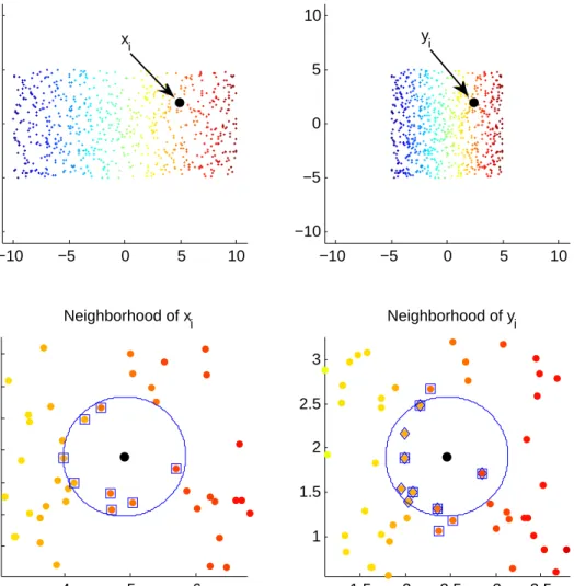
Recent research focuses on assessing dimensionality reduction methods from the geo-metric point of view. In the problem setup in Section 1.2.2, we assumed that ϕ is a local isometry. This assumption implies that the neighboring points in the input space should be mapped to neighbors in the output space, and vice versa for the inverse mapping ψ. This phenomenon can be called “topology preservation”. In order to quantify topology preservation, the following notation will be useful.

Notation

For an observed high-dimensional dataset {x1, . . . ,xn} ⊂ M and a low-dimensional

representation{yb1, . . . ,ybn}, we have the following notation:

• k·k: the Euclidean norm.

dM(·,·): the geodesic distance on the Riemannian manifold M. • |A|: the cardinality of the setA.

• s_ij: the rank of kxi−xjk in ascending order, i.e.

sij =|{k : kxi−xkk ≤ kxi−xjk, 1≤k ≤n}| .

rij: the rank of kyi−yjk in ascending order.

b

(49)

• NI

J(i): the index set of J-nearest neighbors of xi, that is N I J(i) =

n

j|1≤s_ij ≤Jo.

N_JO(i): the index set of J-nearest neighbors of yi, that is N

O J (i) = n j|1≤rbij ≤J o . • N_J(i) = NI J(i) T NO J (i). N∗ J(i) = N I J(i) S NO J (i).

Early attempts to quantify the topology preservation of a dimension reduction method were made in the study of Self-Organizing Maps [Kohonen, 1982]. In order to measure the performance of Self-Organizing Maps, measures such as thetopographic product [Bauer and Pawelzik, 1992],topographic function [Villmann et al., 1997] andquantization error [Kaski and Lagus, 1996] have been developed. Advantages and disadvantages of each method are discussed in detail by P¨olzlbauer [P¨olzlbauer, 2004].

More recently, a few rank-based measures have been proposed, with broader applica-bility. These include mean relative rank errors [Lee and Verleysen, 2007], trustworthiness and continuity [Venna and Kaski, 2001], local continuity meta criterion [Chen and Buja, 2009], and the agreement rate metric [France and Carroll, 2007].

Trustworthiness and continuity (T&C) measures [Venna and Kaski, 2001] are defined by T_J = 1− 1 G_J n X i=1 X j∈NO J(i)\N I J(i) (s_ij −J), C_J = 1− 1 G_J n X i=1 X j∈NI J(i)\N O J(i) (rbij −J), where G_J =        nJ(2n−3J−1) 2 , if J < n/2 n(n−J)(n−J−1) 2 , if J ≥n/2

(50)

is the normalizing factor.

The mean relative rank errors (MRREs) [Lee and Verleysen, 2007] are defined by

MO J = 1− 1 H_J n X i=1 X j∈NO J(i) sij −rbij s_ij , MI J = 1− 1 H_J n X i=1 X j∈NI J(i) sij −rbij b r_ij , whereH_J =nPJ m=1 |n−2m+1|

m is the normalizing factor.

Both T&C and MRREs are restricted to the interval [0,1]. Furthermore, higher values of these measures are desirable properties of algorithms. These two measures try to quantify distinguishably two types of topological errors that occur during the dimension reduction procedures,

(i) non-neighboring points in _Rp _{are mapped by} _ψ_b _{to be neighboring points in}

Rq,

(ii) neighboring points in _Rp _{are mapped by} _ψ_b _{to be non-neighboring points in}

Rq.

These two types of errors create a discrepancy between nearest neighbor ranks in the input and output spaces. Therefore they can be measured by calculating the change of nearest neighbor ranks.

The agreement rate metric (AR) [France and Carroll, 2007] and local continuity meta criterion (LCMC) [Chen and Buja, 2009] are defined similarly:

AR_J = 1 n n X i=1 N O J (i)∩N I J(i) J , LCMC_J = 1 n n X i=1   N O J (i)∩N I J(i) J − J n−1   .

(51)