Hurst, W, Montañez, CAC and Shone, N
Time-Pattern Profiling from Smart Meter Data to Detect Outliers in Energy
Consumption
http://researchonline.ljmu.ac.uk/id/eprint/13655/
Article
LJMU has developed LJMU Research Online for users to access the research output of the University more effectively. Copyright © and Moral Rights for the papers on this site are retained by the individual authors and/or other copyright owners. Users may download and/or print one copy of any article(s) in LJMU Research Online to facilitate their private study or for non-commercial research. You may not engage in further distribution of the material or use it for any profit-making activities or any commercial gain.
The version presented here may differ from the published version or from the version of the record. Please see the repository URL above for details on accessing the published version and note that access may require a subscription.
For more information please contact [email protected]
http://researchonline.ljmu.ac.uk/
Citation
(please note it is advisable to refer to the publisher’s version if you
intend to cite from this work)
Hurst, W, Montañez, CAC and Shone, N (2020) Time-Pattern Profiling from
Smart Meter Data to Detect Outliers in Energy Consumption. IoT, 1 (1). pp.
92-108. ISSN 2624-831X
Article
Time-Pattern Profiling from Smart Meter Data to
Detect Outliers in Energy Consumption
William Hurst1,* , Casimiro A. Curbelo Montañez2 and Nathan Shone3
1 Information Technology Group, Wageningen University and Research, Leeuwenborch, Hollandseweg 1,
6706 KN Wageningen, The Netherlands
2 Owit Iberia S.L., Neàpolis—Rambla de l’Exposició59-69, Vilanova i la Geltrú, 08800 Barcelona, Spain;
3 Department of Computer Science, Liverpool John Moores University, Liverpool L3 3AF, UK;
* Correspondence: [email protected]
Received: 7 August 2020; Accepted: 27 August 2020; Published: 3 September 2020 Abstract:Smart meters have become a core part of the Internet of Things, and its sensory network is increasing globally. For example, in the UK there are over 15 million smart meters operating across homes and businesses. One of the main advantages of the smart meter installation is the link to a reduction in carbon emissions. Research shows that, when provided with accurate and real-time energy usage readings, consumers are more likely to turn offunneeded appliances and change other behavioural patterns around the home (e.g., lighting, thermostat adjustments). In addition, the smart meter rollout results in a lessening in the number of vehicle callouts for the collection of consumption readings from analogue meters and a general promotion of renewable sources of energy supply. Capturing and mining the data from this fully maintained (and highly accurate) sensing network, provides a wealth of information for utility companies and data scientists to promote applications that can further support a reduction in energy usage. This research focuses on modelling trends in domestic energy consumption using density-based classifiers. The technique estimates the volume of outliers (e.g., high periods of anomalous energy consumption) within a social class grouping. To achieve this, Density-Based Spatial Clustering of Applications with Noise (DBSCAN), Ordering Points to Identify the Clustering Structure (OPTICS) and Local Outlier Factor (LOF) demonstrate the detection of unusual energy consumption within naturally occurring groups with similar characteristics. Using DBSCAN and OPTICS, 53 and 208 outliers were detected respectively; with 218 using LOF, on a dataset comprised of 1,058,534 readings from 1026 homes.
Keywords: smart meter; gas; outlier detection; energy; Internet of Things; carbon emission
1. Introduction
Smart meters offer a sustainable flow of energy consumption data (as well as time stamp and user identification) between consumers and utility companies. Information is typically communicated back to the supplier at 30-min intervals. As a capstone technology, smart meters offer a more resilient energy grid management process. Information can be mined and employed for decision-making processes that ultimately allow for the optimisation of the infrastructure management. However, a significant amount of research also exists (some of which is presented in this paper) on how the data collected from the smart meters can be used to detect energy usage patterns in residential homes via user profiling techniques [1]. There are close synergies between the level of fuel consumption and the behaviour of the occupants within their homes [2].
IoT2020,1 93
Analysing the consumption patterns collected by smart meters at frequent intervals using advanced data analysis techniques, provides a practical solution as a smart home Internet of Things (IoT) application for modelling behavioural patterns. For example, Amri et al. used k-means to provide insight into seasonal consumption patterns [3]. Similarly, Palaniappan et al., conducted activity recognition in a home setting [4]. The authors employed a multi-class support vector machine (SVM) for recognising the normal activities, with anomalous behaviours detected by ruling out all possible activities that could be performed from the current activity. The system is focused on identifying anomalous patterns with a lower computational time. Several other fields have also benefitted from the application of anomaly detection using smart meter data, including intrusion detection and fraud detection, in order to identify patterns in the data that differ or stand out from the norm [1]. Also known as anomalies or outliers, these unexpected behaviours are researched actively within the smart grid domain [5,6].
In this paper, we demonstrate how independent user models, when combined, can be used to identify anomalous energy consumption points within granular datasets. These anomalous points can be fed back to the homeowner (or utility provider) as key indicators of either high emissions or overly high consumption, which may affect the billing. The advantage of using outlier detection for this approach is that the anomalous behavioural points detected are based off(1) the user groups’ unique consumption trends (rather than a population-based average); and (2) the homeowners’ unique trend. This is an advantageous approach. Unlike supervised methods, such as classification and regression, clustering analysis does not require label data. Instead, the algorithms use similarity between data features to group them into clusters. This means that anomalous points detected are outliers when compared with both (1) the users’ typical trends and (2) others within a similar social cluster. The general principle of clustering algorithms relies on maximisation of intra-cluster similarities and minimisation of intercluster similarities, where similarity represents a characterisation of the ratio of the number of attributes that a pair of objects share in common, compared to the total amount of attributes between them. As such, the proposed approach is able to detect consumption outliers, when compared with both similar homes and similar users, within the same area and time period. This caters for the detection of homes, or periods of time, in which an individual household generates carbon emissions that are higher than those of a comparable size and location. To the best of our knowledge, this is the first time that a density-based clustering comparison has been conducted with the dataset presented in this paper, to investigate user behaviour using domestic energy consumption monitored via smart meters. Other approaches have been applied, for example, Khan et al. also employed the Irish Social Science Data Archive (ISSDA) smart meter electrical dataset [7] as the focus of their research, but the emphasis was on electricity and load forecasting [8]. Furthermore, this research focuses on gas smart meter only, where the majority of research in the area of smart meter profiling concentrates on electricity meter data [9–11].
The remainder of this paper is as follows. Section2presents an examination of smart meter data and a discussion on related research. Section3provides a case study into density-based clustering techniques that can be applied to a smart meter dataset, and Section4presents a discussion on the results. The paper is concluded in Section5.
2. Background
In 2008, less than 4% of the electricity meters in the world were smart meters. By 2012, the percentage had grown to over 18% and it is expected to rise to 55% by the end of 2020, which is an estimated 800 million in total [5]. This advanced IoT network of smart meters provides a novel gateway into the home, opening up emerging areas of innovative research including human activity profiling, home automation, load management, Non-Intrusive Load Monitoring (NILM), appliance efficiency monitoring, and energy theft [12].
2.1. Smart Meter Data
Smart meters, like many other IoT sensor networks, generate large amounts of data that is often fragmented and complex. In this section, a discussion on smart meter data is put forward using the Irish Commission for Energy Regulation (CER) Gas Smart Meter dataset as an example [13]. The dataset is granular and has the advantage of being accompanied by a post- and pre-evaluation survey of the consumers during the smart meter rollout trial. In result, the consumption readings can be filtered based on categories such as social class, age, gender, opinion on smart meters, cooker type, etc. The social class definitions are presented in Table1. The information displays the official governmental
guidance for outlining which class the occupants belong to, founded on the income of the property owner. There are six classes within the dataset, including anRclass, referring to participants who chose to refuse to provide an answer (other existing social science datasets analyse social classes in greater granularity) [14].
Table 1.Social Class Definitions.
Class Description
AB Advanced managerial/administrative or professional employment.
C1 Supervisory, clerical and junior managerial, administrative, professional occupations
C2 Skilled labour professions
DE Semi-skilled or unskilled manual employment (or currently unemployed)
F Farmers
Refused Refused to respond to question.
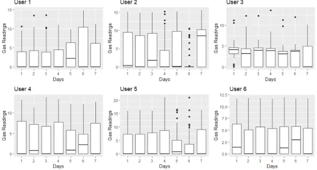
The general supply of gas consumption daily is calculated in kW/h (Kilo Watts per Hour). Gas bills display usage in kWh, despite gas meters measuring cubic metres. In Figure1, a visualisation of the gas meter readings for six random users over a seven-day period is demonstrated. Thex-axis displays days of the week and the raw usage reading is displayed on they-axis. Although rudimentary, the visualisations demonstrate high-level trends in the data consumption patterns. The boxplots display the variation in the usage trend for each of the users. The spacing refers to the degree of dispersion of the gas consumption. The black dots for each user represent outliers. Yet, in the overall dataset, these outliers may be acceptable, depending on trends of similar socio-demographic types. Detecting anomalies is a challenge, without the use of advanced data analytics (such as density-based classification) as a supporting metric for identifying outliers with any confidence and on a mass scale.
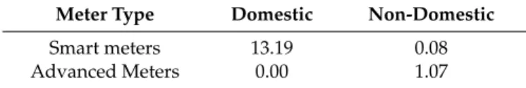
However, there are temporal constraints when proposing an autonomous smart system [15] based on real-time analytics, particularly with regards to supervised classification algorithms. Supervised learning has feature extraction, training and labelling requirements that can be computationally expensive when operating in a live setting. As of 22 May 2019, there were 15,319,200 smart meters installed in the UK (6,611,900 gas and 8,707,300 electric) [16]. The vast majority of the devices are domestic [16], as displayed in Table2. Meaning, it is a significant challenge for supervised learning techniques to be able to operate in real time and remain scalable.
Table 2.2019 Smart Meter Distribution Statistics.
Meter Type Domestic Non-Domestic
Smart meters 13.19 0.08
Advanced Meters 0.00 1.07
However, many related works in this domain do not have real-time requirements, meaning supervised classification techniques are ideal and have been implemented extensively. In the following section, related works are discussed.
IoT2020,1 95
IoT 2019, 2 FOR PEER REVIEW 3 of the consumers during the smart meter rollout trial. In result, the consumption readings can be filtered based on categories such as social class, age, gender, opinion on smart meters, cooker type, etc. The social class definitions are presented in Table 1. The information displays the official governmental guidance for outlining which class the occupants belong to, founded on the income of the property owner. There are six classes within the dataset, including an R class, referring to participants who chose to refuse to provide an answer (other existing social science datasets analyse social classes in greater granularity) [14].
Table 1. Social Class Definitions.
Class Description AB Advanced managerial/administrative or professional
employment.
C1 Supervisory, clerical and junior managerial, administrative, professional occupations
C2 Skilled labour professions
DE Semi-skilled or unskilled manual employment (or currently unemployed)
F Farmers
Refused Refused to respond to question.
The general supply of gas consumption daily is calculated in kW/h (Kilo Watts per Hour). Gas bills display usage in kWh, despite gas meters measuring cubic metres. In Figure 1, a visualisation of the gas meter readings for six random users over a seven-day period is demonstrated. The x-axis displays days of the week and the raw usage reading is displayed on the y-axis. Although rudimentary, the visualisations demonstrate high-level trends in the data consumption patterns. The boxplots display the variation in the usage trend for each of the users. The spacing refers to the degree of dispersion of the gas consumption. The black dots for each user represent outliers. Yet, in the overall dataset, these outliers may be acceptable, depending on trends of similar socio-demographic types. Detecting anomalies is a challenge, without the use of advanced data analytics (such as density-based classification) as a supporting metric for identifying outliers with any confidence and on a mass scale.
Figure 1. Boxplot for Six Random Users.
Figure 1.Boxplot for Six Random Users. 2.2. Related Work
To date, anomaly detection strategies have played a key role in identifying energy fraud in smart meters by analysing historical data [17]. Energy providers identify anomalous consumption patterns and impede energy fraud using consumer’s load profiles, where anomalies are typically classed into three main categories: (1) point anomalies, (2) contextual anomalies and (3) collective anomalies. The first case considers an anomaly when an individual event instance differs when compared with the rest of the data (the approach adopted in this paper). The second type, context anomalies, assume that an event might be considered an anomaly if it occurs in a specific context or circumstances. Finally, collective anomalies represent a collection of different events instances, instead of an individual event as in the two previous cases of anomalies.
For example, energy theft and defective meters have been studied in [18] by means of an anomaly detection framework, aiming at reducing costs and revenue losses in smart grids. The authors use linear programming to model the amount of stolen energy at a particular smart meter as an anomaly coefficient. This is done by enumerating service areas with a high likelihood of theft based on the anomalies detected (reading discrepancies) at the distribution transformer. The proposed framework is capable of detecting meter anomalies even in cases of the random occurrence of theft or faulty equipment.
Other context aware approaches for anomaly detection used in literature are data mining-based, including clustering and association rule-learning techniques. B. Rossi et al. investigated the detection of anomalous behaviour in smart meter data streams using Association Rule Mining (ARM) and categorical clustering silhouette thresholding [19]. ARM is an unsupervised technique that identifies relationships between variables, using strong rules and thresholds to prune redundant information. The technique uncovers rules in large series of events (smart meter readings) to predict the occurrence of an item based on the occurrence of others. The proposed approach is based on aspects of collective and contextual anomalies, proving that single point anomaly detection is not sufficient to determine anomalous events. Potential anomalies identified with ARM are then validated using a clustering silhouette.
K-means-based fuzzy clustering was performed in [20] in order to group consumers with similar Key Performance Indicators (KPI) profiles. This was carried out using 150,000 customers’ energy consumption patterns, where the KPI values were associated using the k-means algorithm. Using their approach, it is possible to identify customers with a high level of use. However, there is a dependence
on the use of KPIs to form correlation. K-means is typically a popular k-partitioning clustering algorithm that represents a centroid as the arithmetic mean of the points in a cluster [21]. Its principle relies on partitioning a given set of observations N into a number of clustersk, where each observation fit to the cluster with the nearest mean. That is, a point is included in a cluster if it is closer to that cluster’s centroid than any other centroid. Giving a training setx(1),. . . ,x(m), each observation is a d-dimensional vectorx(i)∈Rn. Thus, the goal is to predictkcentroids and a labelc(i)for each data point.
The k-mean clustering process can be described as follows; (1) Randomly initialise cluster centroidsµ1, µ2,. . .,µk∈Rnand (2) Repeat until convergence: For everyi, set
c(i):=argmin
j
kx(i)−µjk2 (1)
For everyj, set
µj= Pm i=11 n c(i)= jo x(i) Pm i=11 n c(i)= jo (2)
Despite its popularity, k-means is a non-deterministic algorithm, which means that in every iteration it starts with a random set of centres and converges to a different local minimum each time. K-means is not adopted in this paper during the experimentation. This is because an advantage of density-based clustering is its ability to deal with clusters without assuming that clusters in the data exhibit some type of convex shape naturally, i.e., hyper-spherical or hyper-elliptical, typical from parametric approaches such as nearest-neighbour based. While k-means requires the user to specify the number of clusters to be found, density-based clustering techniques do not assume parametric distributions, are capable of discover arbitrarily-shaped clusters with no previous knowledge about the number of clusters (k), and can handle various amount of noise (anomaly detection). This makes this type of techniques ideal for smart meter data, separating anomalies from what appears to be normal behaviour, especially if there is no further knowledge concerning the nature of the anomalies in the dataset under investigation.
Density-based clustering methods, such as Gaussian Mixture Model (GMM) and density-based spatial clustering of applications with noise (DBSCAN), have been compared in [17] to detect abnormal electricity patterns to challenge electricity theft. These types of unsupervised algorithms group elements into categories, also known as clusters, based on their similarities. The authors proposed a new density-based abnormal detection technique and compared it against k-means, GMM and DBSCAN for identifying electricity theft via smart meter data. Since data with labelled electricity theft information is challenging to obtain, the authors created their own synthetic dataset using six abnormal load profiles and 5000 normal load profiles from residential and commercial users. The proposed clustering-based technique outperformed the other models and detected electricity theft based on the abnormal profiles. Song et al. however, focused on non-invasive energy-use profiles to categorise households into personalised groups [2]. There are similarities with the work presented in this paper, as clustering techniques are used for the grouping. However, the techniques in [2] focus on k-means, hierarchical clustering and self-organising maps, rather than the density-based classification techniques adopted in this paper. An overview of the background research is presented in Table3, which outlines the advantages/disadvantages of each approach.
IoT2020,1 97
Table 3.Synopsis of Related Work.
Authors Method (Type of Analysis) Overview
Song, K. et al., [2]
Personalised energy categorisation through k-means, hierarchical clustering and self-organising maps.
Energy-use profiles employed for the categorisation of households into personalised groups. However, a k
value must be pre-defined. Zheng, K. et al., [17] Density-based clustering methods
(GMM and DBSCAN).
The detection of abnormal electricity patterns to counter electricity theft. The disadvantage is that simulation data is employed for the testing. Yip, S.C. et al., [18] Energy fraud detection using
linear programming.
Reducing costs and revenue losses, with a focus on stolen energy, rather than
carbon reduction. Rossi, B. et al., [19]
Anomaly detection by means of ARM and categorical clustering
silhouette thresholding.
The identification of relationships between variables, to detect collective
and contextual anomalies. Lindèn, M. et al., [20] Outlier Detection using k-means
based fuzzy clustering.
The grouping of consumers to identify customers with a high level of use.
The approach requires the determination of a k value.
GMM, Gaussian Mixture Model; DBSCAN, Density-Based Spatial Clustering of Applications with Noise; ARM, Association Rule Mining.
3. Investigation Methodology
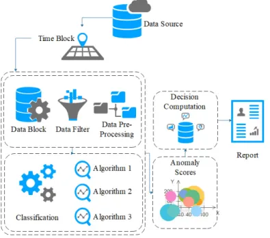
In this section, the methodology is put forward. An autonomous process is advantageous; therefore, a real-time detection model is presented in Figure2and detailed in Algorithm 1.
IoT 2019, 2 FOR PEER REVIEW 6
GMM, Gaussian Mixture Model; DBSCAN, Density-Based Spatial Clustering of Applications with Noise; ARM, Association Rule Mining.
3. Investigation Methodology
In this section, the methodology is put forward. An autonomous process is advantageous; therefore, a real-time detection model is presented in Figure 2 and detailed in Algorithm 1.
Figure 2. Detection Methodology.
Data is collected in blocks using a sliding window approach, where it is pre-processed to check for missing values and passed through the ensemble outlier detection algorithm. The model is a multi-stage process, as in Algorithm 1.
Algorithm 1: Outlier Detection
1. Function dataControl 2. Pass In: data block 3. Function dataManagement 4. Pass In: data block to store
5. Pass Out: data set when complete for data 6. filtering and preProcessing
7. Endfunction 8. Pass In: filteredData 9. Function anomalDectection 10. Pass In: filtered data block 11. send to three classifiers
12. FOR each classifier set anomaly threshold
13. ENDFOR
14. Pass Out: anomalyScores 15. Endfunction
16. Endfunction
17. Function decisionComputation 18. Pass In: Anomaly Scores 19. Pass out: evaluation of outliers 20. IF > anomaly threshold THEN
Figure 2.Detection Methodology.
Data is collected in blocks using a sliding window approach, where it is pre-processed to check for missing values and passed through the ensemble outlier detection algorithm. The model is a multi-stage process, as in Algorithm 1.
Density-based clustering approaches, such as the ones chosen in this methodology (DBSCAN, Ordering Points to Identify the Clustering Structure (OPTICS) and Local Outlier Factor (LOF)), overcome stability concerning the optimal choice of k, as it occurs with k-means.
Algorithm 1:Outlier Detection 1.FunctiondataControl 2. Pass In: data block 3. FunctiondataManagement 4. Pass In: data block to store
5. Pass Out: data set when complete for data 6. filtering and preProcessing
7. Endfunction
8. Pass In: filteredData 9. FunctionanomalDectection 10. Pass In: filtered data block 11. send to three classifiers
12. FOReach classifier set anomaly threshold
13. ENDFOR
14. Pass Out: anomalyScores 15. Endfunction
16.Endfunction
17.FunctiondecisionComputation 18. Pass In: Anomaly Scores 19. Pass out: evaluation of outliers 20. IF>anomaly thresholdTHEN
21. Log Time/User to report 22. ELSEgo to next time period 23. ENDIF
24.Endfunction
3.1. Density-Based Spatial Clustering of Applications with Noise (DBSCAN)
The DBSCAN algorithm and other centroid-based clustering techniques, including k-means, share computational similarities. However, DBSCAN differs in several points. It identifies clusters based on the density of the data points in the feature space instead of using the location of the centroids as conducted by k-means. These facilitate a more accurate identification and separation of the clusters that are of different sizes and shapes, especially convex-shaped data clusters. A second advantage of DBSCAN is its ability to separate noisy data points (outliers) when they are too dissimilar to the rest of the data points. Additionally, instead of randomly selecting the initial locations of the cluster centroids, the DBSCAN algorithm uses a deterministic approach [22].
Unlike other clustering algorithms, DBSCAN only has two input parameters: Epsilon and minimum points, without requiring any other parameters such as the number of clusters in the data set [18]. For two arbitrary data points,pandq, in a data set, and an arbitrary radius Epsilon (εoreps), theε-neighbourhood of a data pointpis Nε(p). Therefore:
Nε(p) = q
d(p,q)< ε (3)
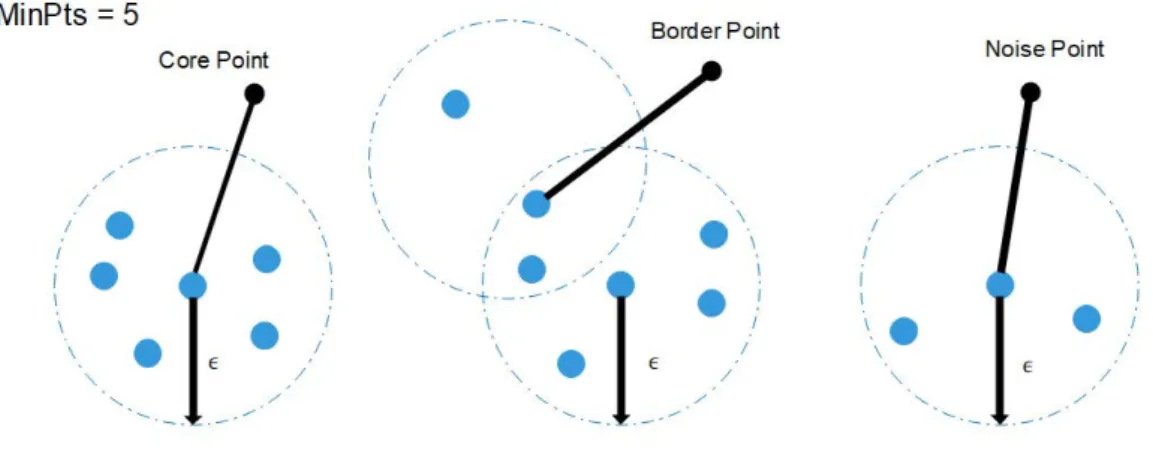
wheredis some distance andε∈R+. On the other hand, the threshold parameter minimum points (MinPts) represents the minimum number of neighbours withinepsradius. The algorithm DBSCAN then uses these two parameters to detect dense regions and classify the available points into core, border and noise points [23].
In the smart meter data, the aim is to identify dense regions measured by the number of objects close to a given point. Parameter estimation is a fundamental task and the first consideration in analysing the smart meter data. Any pointpin the data set with|Nє(p)|≥MinPtsis classified as a core point. We say thatpis a border point, if the number of its neighbours is<MinPts, but it is within the radius of some core pointq. Finally, a point is considered a noise point or an anomaly if it is neither
IoT2020,1 99
a core nor a border point. Therefore, DBSCAN labels the data points as core, border, and anomaly points, as shown in Figure3.
Figure 3.DBSCAN Overview.
Points create clusters with other points that are reachable within itsepsradius. Hence, two points are directly density reachable ifpis a core point andqis in itsє-neighbourhood. If directly density-reachable points are chained together, larger clusters can be established.
DBSCAN has several advantages: (1) Unlike K-means, DBSCAN does not require the user to specify the number of clusters to be generated; (2) DBSCAN can find any shape of clusters. No need for the cluster to be circular; (3) DBSCAN can identify outliers.
A density-based cluster is defined as a group of density connected points. The algorithm DBSCAN works as follow:
1. For each point p in a data set, compute the distance between p and any other point. Then the algorithm finds all neighbour points within a distance eps of the starting point (p). Each point, with a neighbour count greater than or equal to MinPts, is marked as core point.
2. For each core point, if it is not already assigned to a cluster, create a new cluster. Find recursively all its density-connected points and assign them to the same cluster as the core point.
3. Iterate through the remaining unchecked points in the data set.
Those points that do not belong to any cluster are treated as outliers or noise. However, DBSCAN is sensitive to the choice ofeps. This represents a limitation particularly if clusters have different densities. Forepsvalues too small, sparser clusters will be defined as noise. Conversely, forepsvalues too large, denser clusters may be merged together. This implies that, if there are clusters with different local densities, then a singleepsvalue may not suffice.
3.2. OPTICS: Ordering Points to Identify the Clustering Structure
Ordering points to identify the clustering structure (OPTICS) is a generalisation of DBSCAN used to identify density-based clusters in spatial data. It addresses the aforementioned limitation in scenarios where detecting clusters of varying density is important, but keeping the core density-reachable concept from DBSCAN. Unlike DBSCAN, OPTICS is an augmented ordering algorithm that allows flat or hierarchical clustering to be derived from it.
To achieve the detection of meaningful clusters in data of varying density, data points are linearly ordered such that spatially closest points become neighbours in the ordering. As in DBSCAN, OPTICS requires two parameters,epsandMinPts, to describe the maximum distance (radius) to consider and to set the number of points required to form a cluster respectively. However, theepsparameter is only utilised by the algorithm for runtime complexity reduction. Although OPTICS does not produce
IoT2020,1 100
clusters explicitly, it can be used to represent density-based clustering structures from an ordering of data points.
Two additional parameters are introduced in the OPTICS algorithm, core-distance and reachability-distance [24]. The core-distance of a pointprepresents the smallest distance betweenp and a point in itsε-neighbourhood such thatpwould be a core point.
On the other hand, reachability-distance of a pointpwith respect to another pointois the smallest distance such thatpis directly density-reachable fromoifois a core object [25], as depicted in Figure4. 1. For each point p in a data set, compute the distance between p and any other point. Then the algorithm finds all neighbour points within a distance eps of the starting point (p). Each point, with a neighbour count greater than or equal to MinPts, is marked as core point.
2. For each core point, if it is not already assigned to a cluster, create a new cluster. Find recursively all its density-connected points and assign them to the same cluster as the core point.
3. Iterate through the remaining unchecked points in the data set.
Those points that do not belong to any cluster are treated as outliers or noise. However, DBSCAN is sensitive to the choice of eps. This represents a limitation particularly if clusters have different densities. For eps values too small, sparser clusters will be defined as noise. Conversely, for eps values too large, denser clusters may be merged together. This implies that, if there are clusters with different local densities, then a single eps value may not suffice.
3.2. OPTICS: Ordering Points to Identify the Clustering Structure
Ordering points to identify the clustering structure (OPTICS) is a generalisation of DBSCAN used to identify density-based clusters in spatial data. It addresses the aforementioned limitation in scenarios where detecting clusters of varying density is important, but keeping the core density-reachable concept from DBSCAN. Unlike DBSCAN, OPTICS is an augmented ordering algorithm that allows flat or hierarchical clustering to be derived from it.
To achieve the detection of meaningful clusters in data of varying density, data points are linearly ordered such that spatially closest points become neighbours in the ordering. As in DBSCAN, OPTICS requires two parameters, eps and MinPts, to describe the maximum distance (radius) to consider and to set the number of points required to form a cluster respectively. However, the eps parameter is only utilised by the algorithm for runtime complexity reduction. Although OPTICS does not produce clusters explicitly, it can be used to represent density-based clustering structures from an ordering of data points.
Two additional parameters are introduced in the OPTICS algorithm, core-distance and reachability-distance [24]. The core-distance of a point p represents the smallest distance between p and a point in its ε-neighbourhood such that p would be a core point.
On the other hand, reachability-distance of a point p with respect to another point o is the smallest distance such that p is directly density-reachable from o if o is a core object [25], as depicted in Figure 4.
Figure 4. Core distance and reachability distances r(p1,o), r(p2,o) for MinPts = 05.
OPTICS has two main cluster extraction methods based on the ordered reachability structure that the algorithm produces: ExtractDBSCAN and Extract-ξ. The first method performs a clustering equivalent extraction to DBSCAN, whereas the second method identifies clusters hierarchically, using the ordering produced by OPTICS, describing the relative magnitude of cluster density changes (i.e., reachability). 3.3. LOF: Local Outlier Factor
Figure 4.Core distance and reachability distances r(p1,o), r(p2,o) for MinPts=05.
OPTICS has two main cluster extraction methods based on the ordered reachability structure that the algorithm produces: ExtractDBSCAN and Extract-ξ. The first method performs a clustering equivalent extraction to DBSCAN, whereas the second method identifies clusters hierarchically, using the ordering produced by OPTICS, describing the relative magnitude of cluster density changes (i.e., reachability).
3.3. LOF: Local Outlier Factor
The LOF algorithm considers the relative density of points, and detects anomalous values (local outliers) by calculating the local deviation of a data point when compared with its neighbours [26]. This makes the algorithm ideal for application on a dataset where multiple individual types are present. LOF also tends to be advantageous over other proximity-based techniques, LOF employs the relative density of a coefficient against its neighbours. In order to estimate local density, LOF shares properties such as core-distance and reachability-distance with DBSCAN and OPTICS.
The LOF calculation process takes place over five phases including (i) calculating the k-distance, which is the Euclidian distance of the k-th nearest object from an object p; (ii) the construction of the k-nearest neighbour set kNN(p), which is formed by objects within k-distance from p; (iii) computing the reachability distance for p (to an object o), as defined in (4) [27], given that d(p,o) is Euclidian distance of p to o,
reachability−distancek(p,o) =max
k−distance(o), d(p,o) (4) (iv) and the local reachability density (lrd), as in (5),
lrdk(p) =
k P
o∈kNN(p)reachability−distance(p,o)
(5) (v) the final computation for p is,
LOF(p) = 1 k P o∈kNN(p)lrdk(o) lrdk(p) (6)
IoT2020,1 101
4. Results
In this section, an analysis of a smart meter dataset, selected from the CER Smart Metering Trial [13], is assessed. The dataset used for the evaluation is comprised of 1026 users’ gas meter readings over one month. From this, the AB, C1, C2 and DE classes are selected (as the Farmers and Refused class datasets are minor), which filters the total number of users down from 1026 to 1009 (AB: 251, C1: 305, C2: 207, DE: 246, F: 6, Refused: 11). The raw data is used in the experimentation (i.e., without feature extraction) as this is closer to the data obtained for requiring processing in real-time.
4.1. Optimal Parameter Selection
Partitioning methods (K-means, PAM clustering) and hierarchical clustering are suitable for finding spherical-shaped clusters or convex clusters. In other words, they work efficiently only for compact and well separated clusters. Moreover, they are also severely affected by the presence of noise and outliers in the data. Real life data can contain: (i) clusters of arbitrary shape (i.e., oval, linear and “S” shape clusters); (ii) numerous outliers and noise. As previously outlined, identifying clusters with arbitrary shapes using k-means is a challenge. The advantage of DBSCAN, OPTICS and LOF is that they do not require the number of clusters to be specified beforehand by the user.
The DBSCAN algorithm requires users to specify the optimal neighbourhood radiusepsvalue and theMinPtsparameter, which is the minimum number of points within a group to be considered as a cluster. The optimalepsvalue is determined by computing the k-nearest neighbour distances in a matrix of points [23]. To do this, the average of the distances of every point to its k nearest neighbours is calculated. The value of k is specified by the user and corresponds toMinPts.
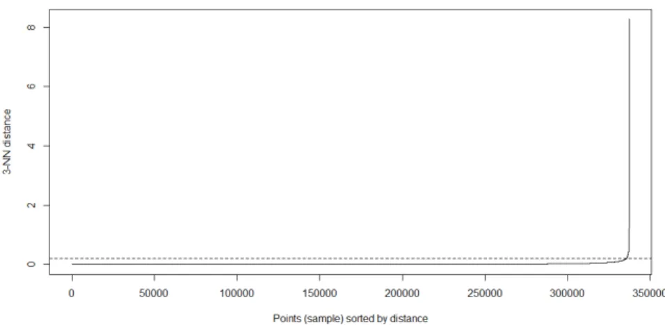
Next, these k-distances are plotted in an ascending order. This is referred to as the elbow method, which corresponds to the optimalepsparameter. The elbow corresponds to a threshold where a sharp change occurs along the k-distance curve. Therefore, following this strategy, an optimalepsvalue of 2.1 is derived from Figure5(identified by the ab-line); the minimum number of points (MinPts) is set to 3. OnceepsandMinPtsare defined, DBSCAN divides the data points into core, border and outlier points. The algorithm starts by selecting points that are not assigned to a cluster and calculates its neighbour
within a distanceIoT 2019, 2 FOR PEER REVIEW eps. 10
Figure 5. Optimal radius (eps) Calculation. 4.2. DBSCAN
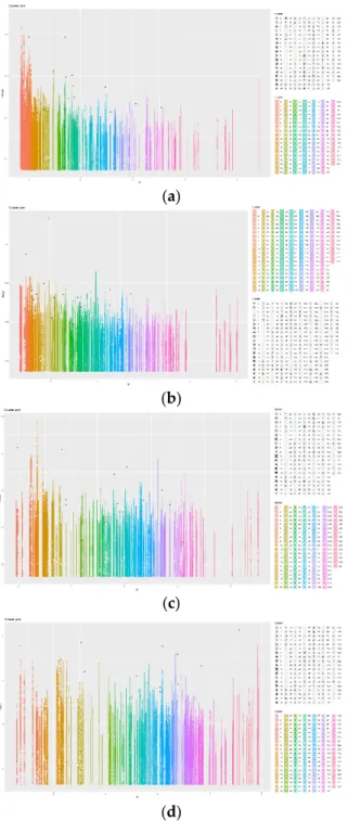
Points with neighbour counts equal to or greater than MinPts are marked as core points and clusters are created around them. Thus, points that do not fit any of the clusters are considered outliers by DBSCAN. Using the optimal eps parameter derived from Figure 4 and MinPts = 3, the results are presented in Table 4 and Figure 6 (where the black dots are the outliers). Out of a total 1,058,534 points, DBSCAN identified 564 clusters and 53 anomaly points.
(a) (b)
(c) (d)
Figure 6. DBSCAN Visualisation (a) AB, (b) C1, (c) C2, (d) DE. Table 4. DBSCAN Output.
Class Objects Clusters Noise
AB 337344 124 16 C1 409920 173 15 C2 278208 135 10 DE 330624 132 12
Total 1,058,534 564 53
Figure 5.Optimal radius (eps) Calculation. 4.2. DBSCAN
Points with neighbour counts equal to or greater thanMinPtsare marked as core points and clusters are created around them. Thus, points that do not fit any of the clusters are considered outliers by DBSCAN. Using the optimalepsparameter derived from Figure4andMinPts=3, the results are presented in Table4and Figure6(where the black dots are the outliers). Out of a total 1,058,534 points, DBSCAN identified 564 clusters and 53 anomaly points.
BSCAN identified 564 clusters and 53 anomaly points.
(a)
(b)
(c)
(d)
Figure 6. DBSCAN Visualisation (a) AB, (b) C1, (c) C2, (d) DE.
Table 4. DBSCAN Output.
Class Objects Clusters Noise AB 337344 124 16 C1 409920 173 15 C2 278208 135 10 DE 330624 132 12 Total 1,058,534 564 53 4.3. OPTICS
Figure 6.DBSCAN Visualisation (a) AB, (b) C1, (c) C2, (d) DE. 4.3. OPTICS
OPTICS addresses one of the DBSCAN deficiencies, in that it detects meaningful clusters within data that has varying density. However, this also means that it is a more memory-expensive algorithm. In this section, the results obtained using the OPTICS algorithm are presented. First, results extracted using extractDBSCAN are presented. It is possible to plot directly the density-based order produced by the algorithm as a reachability plot (Figure7). In such plots, low reachability-distances are depicted as valleys representing clusters separated by peaks, which represent points with larger distances. The example displayed in Figure7is for the AB social class. Based on the graph, theepsis set at 1 for optics as the median value between the peaks and valleys.
IoT2020,1 103
IoT 2019, 2 FOR PEER REVIEW 11 4.3. OPTICS
OPTICS addresses one of the DBSCAN deficiencies, in that it detects meaningful clusters within data that has varying density. However, this also means that it is a more memory-expensive algorithm. In this section, the results obtained using the OPTICS algorithm are presented. First, results extracted using extractDBSCAN are presented. It is possible to plot directly the density-based order produced by the algorithm as a reachability plot (Figure 7). In such plots, low reachability-distances are depicted as valleys representing clusters separated by peaks, which represent points with larger distances. The example displayed in Figure 7 is for the AB social class. Based on the graph, the eps is set at 1 for optics as the median value between the peaks and valleys.
Figure 7. Ordering Points to Identify the Clustering Structure (OPTICS) Reachability Plot.
From the 1,058,534 points, OPTICS classified 208 anomaly points and identified 794 clusters in the overall dataset. AB is classed with 191 clusters and 60 outlier points; C1 and C2 with 235 and 178 clusters, and 59 and 43 anomalous points, respectively. DE has 190 clusters and 46 anomalies, as outlined in Table 5.
Table 5. OPTICS Output.
Class Objects Clusters Noise
AB 337344 191 60 C1 409920 235 59 C2 278208 178 43 DE 330624 190 46
Total 1,058,534 794 208
A sample of reachability distance and core distance values produced by OPTICS are presented in Table 6, where the first column represents the order that OPTICS produces for each data point in x, ReachDist is the reachability distance for each data point in x, CoreDist is the core distance for each data pint in x, and Cluster indicates the assigned cluster labels in the order of the data points in x.
Table 6. OPTICS: Reach Distance and Core Distance.
Order ReachDist CoreDist
1 Inf 0.000444
253,024 0.000217 0.000000
168,968 0.003287 0.000217
84,395 0.000495 0.001004
253,076 0.000000 0.000662
Figure 7.Ordering Points to Identify the Clustering Structure (OPTICS) Reachability Plot.
Table 4.DBSCAN Output.
Class Objects Clusters Noise
AB 337,344 124 16
C1 409,920 173 15
C2 278,208 135 10
DE 330,624 132 12
Total 1,058,534 564 53
From the 1,058,534 points, OPTICS classified 208 anomaly points and identified 794 clusters in the overall dataset. AB is classed with 191 clusters and 60 outlier points; C1 and C2 with 235 and 178 clusters, and 59 and 43 anomalous points, respectively. DE has 190 clusters and 46 anomalies, as outlined in Table5.
Table 5.OPTICS Output.
Class Objects Clusters Noise
AB 337,344 191 60
C1 409,920 235 59
C2 278,208 178 43
DE 330,624 190 46
Total 1,058,534 794 208
A sample of reachability distance and core distance values produced by OPTICS are presented in Table6, where the first column represents the order that OPTICS produces for each data point in x, ReachDist is the reachability distance for each data point in x, CoreDist is the core distance for each data pint in x, and Cluster indicates the assigned cluster labels in the order of the data points in x.
Table 6.OPTICS: Reach Distance and Core Distance.
Order ReachDist CoreDist
1 Inf 0.000444 253,024 0.000217 0.000000 168,968 0.003287 0.000217 84,395 0.000495 0.001004 253,076 0.000000 0.000662 4.4. LOF
The LOF algorithm adopts the same theoretical basis as OPTICS, as LOF orders objects in the dataset in order of their outlier-ness. Therefore, the expectation is that LOF and OPTICS produce
comparable results. The LOF anomaly score is calculated by taking the number of variants. The LOF anomaly score measures the local deviation of density through determining how isolated the value is given by k-nearest neighbours.
Table5can also be visualised as a cluster plot, as shown in the example Figure8. Any point not included within the clusters is treated as an anomaly. Figure8displays the clustering for the AB social class as an example plot, where outliers are represented by black dots.
IoT 2019, 2 FOR PEER REVIEW 12 Table 5 can also be visualised as a cluster plot, as shown in the example Figure 8. Any point not included within the clusters is treated as an anomaly. Figure 8 displays the clustering for the AB social class as an example plot, where outliers are represented by black dots.
Figure 8. Example OPTICS Visualisation for AB Data.
4.4. LOF
The LOF algorithm adopts the same theoretical basis as OPTICS, as LOF orders objects in the dataset in order of their outlier-ness. Therefore, the expectation is that LOF and OPTICS produce comparable results. The LOF anomaly score is calculated by taking the number of variants. The LOF anomaly score measures the local deviation of density through determining how isolated the value is given by k-nearest neighbours.
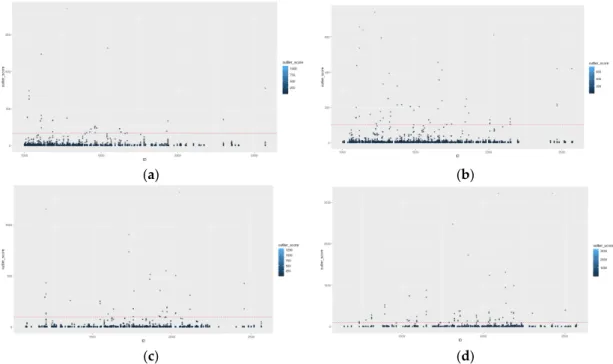
Typically, when a value close to 1 is generated, the indication is that the object is comparable to its neighbours (i.e., inlier). However, a more suitable approach is to define a threshold for the anomaly identification, defined by either (1) an approximate quantile or (2) by using the elbow method. In this approach, we make use of the elbow method to identify 100 as a suitable deviation in the curve. LOF is able to identify 218 anomalies in the dataset. Table 7 presents the highest anomaly score values for the first 10 anomalies, with the results visualised in Figure 9 (User ID is displayed on the x-axis, with the anomaly score on the y-axis. The red line signifies the threshold for anomaly identification).
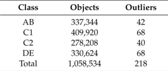
Table 7. Local Outlier Factor (LOF) Output.
Class Objects Outliers AB 337344 42
C1 409920 68 C2 278208 40 DE 330624 68 Total 1,058,534 218
Figure 8.Example OPTICS Visualisation for AB Data.
Typically, when a value close to 1 is generated, the indication is that the object is comparable to its neighbours (i.e., inlier). However, a more suitable approach is to define a threshold for the anomaly identification, defined by either (1) an approximate quantile or (2) by using the elbow method. In this approach, we make use of the elbow method to identify 100 as a suitable deviation in the curve. LOF is able to identify 218 anomalies in the dataset. Table7presents the highest anomaly score values for the first 10 anomalies, with the results visualised in Figure9(User ID is displayed on thex-axis, with the anomaly score on they-axis. The red line signifies the threshold for anomaly identification).
IoT 2019, 2 FOR PEER REVIEW 13
(a) (b)
(c) (d)
Figure 9. LOF Visualisation (a) AB, (b) C1, (c) C2, (d) DE. 5. Discussion
Centroid-based methods, such as k-means, require the number of clusters to be specified beforehand, which limits the identification of anomalies. K-means is also not capable of reporting any noise or anomalies. Hence, in this study, k-means was not adopted. Instead, three density-based algorithms were selected: DBSCAN, OPTICS and LOF, which depend on model-specific parameters but do not require the number of clusters to be specified by the user (however, in the case of LOF, an optional k value can be defined and is usually set as a range of values, e.g., 5 to 10). Experiments conducted using DBSCAN allowed the identification of 564 different clusters, as shown in Figure 6.
To achieve this, the optimal radius (eps) was achieved by computing the k-nearest neighbour
distances in a matrix of points. Thus, the eps value was derived from Figure 5 and is equal to 2.1. The
minimum number of points within eps or MinPts was set to 3. Since DBSCAN can have complications
in scenarios with clusters of varying densities, we used the OPTICS algorithm to create clustering equivalent extraction to DBSCAN based on an ordered reachability structure generated by OPTICS. The reachability plot in Figure 6 identified the reachability-distance with the median value selected. Using OPTICS, a higher number of anomalies were detected, creating more compact clusters; 208 data points were considered outliers with 794 clusters. Finally, experiments using LOF were performed, with 218 anomalous points identified. Examples of anomalies found using LOF include User 1277 in the AB data, who had the most significant outlier score; however, user 1030 and user 1620 had the highest number of outlier readings. User 1221 had the two highest anomalous data points in C1. The datasets are essentially split into two clusters, normal points and outliers, defined by the threshold line.
The results obtained with LOF would be comparable in terms of clusters with those achieved with k-means (k = 5) but also similar to the results obtained with OPTICS. However, the results achieved with LOF are somewhat limited, in that the k value range requires refinement; this would be an on-going process. Also, the anomaly threshold must be set by the user, meaning there may be some anomalies missed by the defined cut-off threshold, such as borderline points (for example, User 1958 in the DE data had an anomaly score of 97.19 for one time stamp). However, this can be mitigated through an iterative selection of the optimum threshold using a human-in-the-loop approach. Based on this, the recommendation is to adopt DBSCAN and OPTICS for the detection of high energy usage patterns as there is no requirement for iterative threshold definition and no human-in-the-loop considerations. However, with an iterative refinement, LOF may produce more accurate results over
IoT2020,1 105
Table 7.Local Outlier Factor (LOF) Output.
Class Objects Outliers
AB 337,344 42 C1 409,920 68 C2 278,208 40 DE 330,624 68 Total 1,058,534 218 5. Discussion
Centroid-based methods, such as k-means, require the number of clusters to be specified beforehand, which limits the identification of anomalies. K-means is also not capable of reporting any noise or anomalies. Hence, in this study, k-means was not adopted. Instead, three density-based algorithms were selected: DBSCAN, OPTICS and LOF, which depend on model-specific parameters but do not require the number of clusters to be specified by the user (however, in the case of LOF, an optional k value can be defined and is usually set as a range of values, e.g., 5 to 10). Experiments conducted using DBSCAN allowed the identification of 564 different clusters, as shown in Figure6. To achieve this, the optimal radius (eps) was achieved by computing the k-nearest neighbour distances in a matrix of points. Thus, theepsvalue was derived from Figure5and is equal to 2.1. The minimum number of points withinepsorMinPtswas set to 3. Since DBSCAN can have complications in scenarios with clusters of varying densities, we used the OPTICS algorithm to create clustering equivalent extraction to DBSCAN based on an ordered reachability structure generated by OPTICS. The reachability plot in Figure6identified the reachability-distance with the median value selected. Using OPTICS, a higher number of anomalies were detected, creating more compact clusters; 208 data points were considered outliers with 794 clusters. Finally, experiments using LOF were performed, with 218 anomalous points identified. Examples of anomalies found using LOF include User 1277 in the AB data, who had the most significant outlier score; however, user 1030 and user 1620 had the highest number of outlier readings. User 1221 had the two highest anomalous data points in C1. The datasets are essentially split into two clusters, normal points and outliers, defined by the threshold line.
The results obtained with LOF would be comparable in terms of clusters with those achieved with k-means (k=5) but also similar to the results obtained with OPTICS. However, the results achieved with LOF are somewhat limited, in that the k value range requires refinement; this would be an on-going process. Also, the anomaly threshold must be set by the user, meaning there may be some anomalies missed by the defined cut-offthreshold, such as borderline points (for example, User 1958 in the DE data had an anomaly score of 97.19 for one time stamp). However, this can be mitigated through an iterative selection of the optimum threshold using a human-in-the-loop approach. Based on this, the recommendation is to adopt DBSCAN and OPTICS for the detection of high energy usage patterns as there is no requirement for iterative threshold definition and no human-in-the-loop considerations. However, with an iterative refinement, LOF may produce more accurate results over a longer duration than DBSCAN and OPTICS. Therefore, there is a trade-offconsideration in terms of time vs. efficiency. In Table8, a comparison of the results obtained by the density-based clustering algorithm in terms of number of clusters and anomalies identified is provided.
Table 8.OPTICS.
Algorithm Parameters # Clusters Anomaly Points
DBSCAN Eps=2.1,MinPts=3 564 53
OPTICS Eps=1 794 208
As observed from the different experiments conducted in this study, each clustering algorithm reported various outcomes using the same smart meter dataset. The fact that each algorithm requires specific parameters to model the clusters is a result of theepsselection. Theepsdecision also affects the anomaly detection process, so the identification of theepsis paramount in the detection of anomalous points. Additionally, the identified clusters may ultimately show how users perform based on their lifestyle and social behaviours, which could allow to label domestic energy consumption by social clusters and high energy consumption points.
The comparison provided in the paper can help researchers to label anomaly points in unlabelled smart meter/IoT data for further machine learning (ML) studies (i.e., classification experiments). This should also be highlighted in future work and can ultimately help to categorise anomalies in residential energy consumption. When compared with k-means and other partition-based clustering methods, density-based clustering techniques can deal with clusters of arbitrary shape, benefitting the identification of anomalies in the smart meter data where different households will produce different consumption patterns depending on various factors (number of occupants, energy theft and fault detection, among other factors).
In our approach, social classes are factored into the clustering, meaning that outliers are based on similar groupings. Therefore, outliers are detected with respect to similar data trends. The system proposed in the paper also focuses on the identification of point anomalies using density-based clustering, from which the estimate is that between 0.005%–0.020% of points are anomalous. Detecting and eliminating these high consumption points is beneficial. Research shows that if every household adopted more energy efficiency technologies (e.g., a smart meter) it could be possible to achieve an 11% reduction of the 2050 carbon emissions target [28].
In this work, we do not consider tariffbands (although it is considered in other works [29] and can be extracted from the survey data). This is because the goal is to identify outliers in consumption patterns within social groupings, which are high periods of anomalous energy consumption irrespective of the fuel price. Whilst the authors recognise that recommending tariffchange to consumers has tremendous benefits (e.g., for fuel poverty), the aim of this research is to encourage households to change their behavioural trends around the home for reducing carbon emissions, meaning tariff detection is outside of the scope of this research.
6. Conclusions
In this paper, anomaly detection from IoT smart meter data is investigated for the benefits of identifying high consumption trends in domestic energy consumption. Density-based clustering techniques were employed to identify clusters as normal behaviour and noise points as anomalies, based on the different properties of the tested models. The results were produced from the raw data, rather than using a feature extraction process. This was selected as an experimentation approach as the data used is closer to data obtained in a real-time data stream. Also, the elimination of the feature extraction and normalisation process will reduce the pre-processing time for greater efficiency. Therefore, the next immediate stage of this work will involve the comparison of this approach with the same techniques with a feature extraction process employed prior to clustering.
The techniques utilised in the present study function based on distance computation between a pair of data points, assuming therefore that this computation can discriminate between outliers and normal points well enough. However, classification-based techniques may play a better role in situations where identifying optimal distance measure is challenging. Hence, in future work the clusters identified by each classifier will be used as labels to conduct classification tasks using supervised machine learning models, such as artificial neural network (ANN) or support vector machine (SVM); meaning this work can be built on by future researchers. Furthermore, cluster information can be combined with further survey data in order to enhance the insights extracted from the smart meter data. This can bring more opportunities to the field, using the smart metering infrastructure and the
IoT2020,1 107
Internet of Things IoT to, for example, monitor energy usage through appliances interactions to model domestic energy consumption and social class behaviour.
Author Contributions: Individual contributions are as follows, conceptualization, W.H. and C.A.C.M.; methodology, W.H. and C.A.C.M.; software, W.H. and C.A.C.M.; validation, W.H. and C.A.C.M.; formal analysis, W.H. and C.A.C.M.; investigation, W.H. and C.A.C.M.; data curation, W.H. and C.A.C.M.; writing—original draft preparation, W.H., C.A.C.M., and N.S.; writing—review and editing, W.H., C.A.C.M., and N.S.; visualization, W.H. and C.A.C.M.; supervision, W.H.; project administration, C.A.C.M.. All authors have read and agreed to the published version of the manuscript.
Funding:This research received no external funding.
Acknowledgments: The data used in this paper is available for request from the Commission for Energy Regulation (CER). (2012). CER Smart Metering Project—Gas Customer Behaviour Trial, 2009-2010 [dataset]. 1st Edition. Accessed via the Irish Social Science Data Archive. SN: 0013-00.www.ucd.ie/issda/CER-gas.
Conflicts of Interest:The authors declare no conflict of interest. Abbreviations
Abbreviation Explanation
ANN Artificial Neural Network
ARM Association Rule Mining
CER Commission for Energy Regulation
DBSCAN Density-Based Spatial Clustering of Applications with Noise
GMM Gaussian Mixture Model
IoT Internet of Things
ISSDA Irish Social Science Data Archive KPI Key Performance Indicators kW/h Kilo Watts per Hour
LOF Local Outlier Factor
ML Machine Learning
NILM Non-Intrusive Load Monitoring
OPTICS Ordering Points to Identify the Clustering Structure
PAM partition around medoids
SVM Support Vector Machine
References
1. Jain, S.; Choksi, K.A.; Pindoriya, N.M. Rule-based classification of energy theft and anomalies in consumers load demand profile.IET Smart Grid2019,2, 612–624. [CrossRef]
2. Song, K.; Anderson, K.; Lee, S.; Raimi, K.T.; Hart, P.S. Non-Invasive Behavioral Reference Group Categorization Considering Temporal Granularity and Aggregation Level of Energy Use Data.Energies2020, 13, 3678. [CrossRef]
3. Amri, Y.; Fadhilah, A.L.; Fatmawati, N.S.; Rani, S. Analysis Clustering of Electricity Usage Profile Using K-Means Algorithm.IOP Conf. Ser. Mater. Sci. Eng.2016,105, 012020. [CrossRef]
4. Palaniappan, A.; Bhargavi, R.; Vaidehi, V. Abnormal human activity recognition using SVM based approach. In Proceedings of the International Conference on Recent Trends in Information Technology, Chennai, Tamil Nadu, India, 19–21 April 2012.
5. Fenza, G.; Gallo, M.; Loia, V. Drift-Aware Methodology for Anomaly Detection in Smart Grid.IEEE Access
2019,7, 9645–9657. [CrossRef]
6. Zhang, W.; Dong, X.; Li, H.; Xu, J.; Wang, D. Unsupervised Detection of Abnormal Electricity Consumption Behavior Based on Feature Engineering.IEEE Access2020,8, 55483–55500. [CrossRef]
7. Commission for Energy Regulation (CER), Irish Social Science Archive (ISSDA), —CER Smart Metering Project—Electricity Customer Behaviour Trial, 2009–2010 [dataset], Ireland: SN: 0012-00. 2012. Available online:www.ucd.ie/issda/CER-electricity(accessed on 6 August 2020).
8. Khan, Z.A.; Jayaweera, D. Smart Meter Data Based Load Forecasting and Demand Side Management in Distribution Networks with Embedded PV Systems.IEEE Access2019,8, 2169–3536. [CrossRef]
9. Al-Jarrah, Y.; Al-Hammadi, Y.; Yoo, P.D.; Muhaidat, S. Multi-Layered Clustering for Power Consumption Profiling in Smart Grids.IEEE Access2017,5, 18459–18468. [CrossRef]
10. Khan, I.; Huang, J.Z.; Masud, M.A.; Jiang, Q. Segmentation of Factories on Electricity Consumption Behaviors Using Load Profile Data.IEEE Access2016,4, 8394–8406. [CrossRef]
11. Park, K.-J.; Son, S.-Y. A Novel Load Image Profile-Based Electricity Load Clustering Methodology.IEEE Access
2019,7, 59048–59058. [CrossRef]
12. Hock, D.; Kappes, M.; Ghita, B. Entropy-Based Metrics for Occupancy Detection Using Energy Demand. Entropy2020,22, 731. [CrossRef]
13. Commission for Energy Regulation (CER); Irish Social Science Archive (ISSDA). Commission for Energy Regulation (CER)—CER Smart Metering Project—Gas Customer Behaviour Trial, 2009–2010 [dataset], Ireland: Irish Social Science Data Archive. SN: 0013-00. 2012. Available online:www.ucd.ie/issda/CER-gas(accessed on 6 August 2020).
14. National Readership Survey (NRS). Social Grade|National Readership Survey, December 2016. Available online:http://www.nrs.co.uk/nrs-print/lifestyle-and-classification-data/social-grade/(accessed on 4 August 2020).
15. García-Magariño, I.; Nasralla, M.M.; Nazir, S. Real-Time Analysis of Online Sources for Supporting Business Intelligence Illustrated with Bitcoin Investments and IoT Smart-Meter Sensors in Smart Cities.Electronics
2020,9, 1101. [CrossRef]
16. Department for Business, Energy and Industrial Strategy (BEIS), Smart Meter Statistics Report; BEIS: London, UK, 2019. 17. Zheng, K.; Wang, Y.; Chen, Q.; Li, Y. Electricity theft detecting based on density-clustering method. InIEEE
Innovative Smart Grid Technologies—Asia (ISGT-Asia); IEEE: Aukland, New Zealand, 2017.
18. Yip, S.-C.; Tan, W.-N.; Tan, C.; Gan, M.-T.; Wong, K. An anomaly detection framework for identifying energy theft and defective meters in smart grids.Int. J. Electr. Power Energy Syst.2018,101, 189–203. [CrossRef] 19. Rossi, B.; Chren, S.; Buhnova, B.; Pitner, T. Anomaly detection in Smart Grid data: An experience report.
In Proceedings of the IEEE International Conference on Systems, Man, and Cybernetics (SMC), Budapest, Hungary, 9–12 October 2016.
20. Lindèn, M.; Helbrink, J.; Nilsson, M.; Pogosjan, D. Categorisation of electricity customers based upon their demand patterns.CIRED Open Access Proc. J.2017,1, 2628–2631. [CrossRef]
21. Nerurkar, P.; Shirke, A.; Chandane, M.; Bhirud, S. Empirical Analysis of Data Clustering Algorithms. Procedia Comput. Sci.2018,125, 770–779. [CrossRef]
22. Handra, S.I.; Ciocârlie, H. Anomaly detection in data mining. In Hybrid approach between filtering-and-refinement and DBSCAN. In Proceedings of the IEEE International Symposium on Applied Computational Intelligence and Informatics (SACI), Timisoara, Romania, 19–21 May 2011.
23. Hahsler, M.; Piekenbrock, M.; Doran, D. dbscan: Fast Density-based Clustering with R.J. Stat. Softw.2019, 91, 1–30. [CrossRef]
24. Schubert, E.; Gertz, M. Improving the Cluster Structure Extracted from OPTICS Plots. In Proceedings of the Lernen, Wissen, Daten, Analysen (LWDA 2018), Mannheim, Germany, 22–24 August, 2018; pp. 318–329. 25. Ankerst, M.; Breunig, M.M.; Kriegel, H.-P.; Sander, J. OPTICS: Ordering Points to Identify the Clustering
Structure. In Proceedings of the ACM SIGMOD’99 International Conference on Management of Data, Philadelphia, PA, USA, 1–3 June 1999.
26. Vasudevan, A.R.; Selvakumar, S. Local outlier factor and stronger one class classifier based hierarchical model for detection of attacks in network intrusion detection dataset.Front. Comput. Sci.2016,10, 755–766. [CrossRef] 27. Lee, J.; Kang, B.; Kang, S.H. Integrating independent component analysis and local outlier factor for
plant-wide process monitoring.J. Process Control2011,21, 1011–1021. [CrossRef]
28. Smart Energy, G.B. The Missing Piece in Climate Conversations. Available online:https://www.smartenergygb. org/en/smart-living/the-missing-piece-in-the-climate-conversation(accessed on 19 August 2020).
29. Hurst, W.; Montañez, C.A.C.; Shone, N.; Al-Jumeily, D. An Ensemble Detection Model Using Multinomial Classification of Stochastic Gas Smart Meter Data to Improve Wellbeing Monitoring in Smart Cities. IEEE Access2020,8, 7877–7898. [CrossRef]
©2020 by the authors. Licensee MDPI, Basel, Switzerland. This article is an open access article distributed under the terms and conditions of the Creative Commons Attribution (CC BY) license (http://creativecommons.org/licenses/by/4.0/).