High performance computing applications: Inter-process communication, workflow optimization, and deep learning for computational nuclear physics

2018

High performance computing applications:

Inter-process communication, workflow optimization,

and deep learning for computational nuclear

physics

Gianina Alina Negoita

Follow this and additional works at:

https://lib.dr.iastate.edu/etd

Part of the

Computer Sciences Commons

This Dissertation is brought to you for free and open access by the Iowa State University Capstones, Theses and Dissertations at Iowa State University Digital Repository. It has been accepted for inclusion in Graduate Theses and Dissertations by an authorized administrator of Iowa State University Digital Repository. For more information, please [email protected].

Recommended Citation

Negoita, Gianina Alina, "High performance computing applications: Inter-process communication, workflow optimization, and deep learning for computational nuclear physics" (2018).Graduate Theses and Dissertations. 16858.

optimization, and deep learning for computational nuclear physics

by

Gianina Alina Negoita

A dissertation submitted to the graduate faculty in partial fulfillment of the requirements for the degree of

DOCTOR OF PHILOSOPHY

Major: Computer Science

Program of Study Committee: Gurpur M. Prabhu, Major Professor

Soma Chaudhuri Shashi K. Gadia Simanta Mitra James P. Vary

The student author, whose presentation of the scholarship herein was approved by the program of study committee, is solely responsible for the content of this dissertation. The Graduate College will ensure this dissertation is globally accessible and will not permit alterations after a degree is

conferred.

Iowa State University Ames, Iowa

2018

DEDICATION

I would like to dedicate this thesis to my mom Stela, to my dad Alexandru, to my brother Cristian, and to my cat Milly for their love, endless support, and encouragement.

TABLE OF CONTENTS

Page

LIST OF TABLES . . . vi

LIST OF FIGURES . . . vii

ACKNOWLEDGMENTS . . . xii

ABSTRACT . . . xiv

CHAPTER 1. GENERAL INTRODUCTION . . . 1

1.1 Introduction and Background . . . 1

1.1.1 High Performance Computing . . . 2

1.1.2 Machine Learning . . . 21

1.1.3 Nuclear Physics . . . 28

1.2 Thesis Organization . . . 33

References . . . 35

CHAPTER 2. THE PERFORMANCE AND SCALABILITY OF THE SHMEM AND COR-RESPONDING MPI-3 ROUTINES ON A CRAY XC30 . . . 39

2.1 Introduction . . . 40

2.2 Communication Tests and Performance Results . . . 42

2.2.1 Test 1: Accessing Distant Messages . . . 43

2.2.2 Test 2: Circular Right Shift . . . 46

2.2.3 Test 3: Gather . . . 48

2.2.4 Test 4: Broadcast . . . 50

2.3 Summary and Conclusions . . . 54

References . . . 55

2.A Additional Material . . . 62

CHAPTER 3. HPC–BENCH: A TOOL TO OPTIMIZE BENCHMARKING WORKFLOW FOR HIGH PERFORMANCE COMPUTING . . . 69

3.1 Introduction . . . 69

3.2 Tool Design . . . 71

3.3 Example Using HPC–Bench . . . 78

3.4 Conclusion . . . 80

References . . . 90

CHAPTER 4. DEEP LEARNING: A TOOL FOR COMPUTATIONAL NUCLEAR PHYSICS 91 4.1 Introduction . . . 92

4.2 Theoretical Framework . . . 95

4.2.1 Ab Initio NCSM Method . . . 95

4.2.2 Artificial Neural Networks . . . 97

4.3 ANN Design . . . 102

4.4 Results and Discussions . . . 104

4.5 Conclusion and Future Work . . . 112

References . . . 113

CHAPTER 5. DEEP LEARNING: EXTRAPOLATION TOOL FORAB INITIONUCLEAR THEORY . . . 119

5.1 Introduction . . . 120

5.2 Theoretical Framework . . . 122

5.2.1 Ab Initio NCSM Method . . . 122

5.2.2 Artificial Neural Networks . . . 125

5.3 ANN Design and Filtering . . . 128

5.5 Conclusion and Future Work . . . 140

References . . . 142

CHAPTER 6. GENERAL CONCLUSIONS . . . 148

LIST OF TABLES

Page

Table 2.1 Average over all ranks of the median times in milliseconds (ms) for the ‘accessing distant messages’ test. . . 46

Table 3.1 The R dataframe generated with the code from Figure3.9for 8-byte message size for application 2. . . 77

Table 4.1 Comparison of the ANN predicted results with results from the current best upper bounds and from other estimation methods. . . 111 Table 4.2 The MSE performance function values on the training and testing data sets

and on theNmax= 12,14,16,and 18 data set. . . 112

Table 5.1 Comparison of the ANN predicted results with results from the current best upper bounds and from other extrapolation methods, such as Extrapolation Aa [6] and Extrapolation B [3,4], with their uncertainties. The experimen-tal gs energy is taken from [40]. The experimenexperimen-tal point-proton rms radius is obtained from the measured charge radius by the application of electro-magnetic corrections [41]. Energies are given in units ofM eV and radii are in units of femtometers (f m). . . 138

LIST OF FIGURES

Page

Figure 1.1 The topology of a compute node on the student cluster at Iowa State Uni-versity. . . 3 Figure 1.2 TheDragonfly topology for the interconnection network for NERSC’s

“Edi-son” Cray XC30. Image courtesy of NERSC [1]. . . 5 Figure 1.3 The topology of a compute node for NERSC’s “Edison” Cray XC30. Image

courtesy of NERSC [1]. . . 6 Figure 1.4 Detailed hierarchical map for the topology of a compute node for NERSC’s

“Edison” Cray XC30. Image courtesy of NERSC [1]. . . 7 Figure 1.5 A schematic diagram of remote memory access using a window object

cre-ated withmpi win allocate for MPI get and put. . . 13 Figure 1.6 The three synchronization mechanisms for one-sided communication in MPI.

The arguments indicate the target rank, wherei6=j 6=k. . . 14 Figure 1.7 A schematic diagram of symmetric objects for SHMEM. . . 15 Figure 1.8 A schematic diagram of remote memory access using a symmetric object for

SHMEMget and put. . . 16 Figure 1.9 PE 0 ‘gets’ a message from PE i, wherei6= 0 using the shmem get routine. 17 Figure 1.10 PEi ‘puts’ a message on PE 0, wherei6= 0 using the shmem put routine. . 18 Figure 1.11 An example for the HPC workflow using n applications that are run on p

processes. . . 20 Figure 1.12 An example of afeed-forward multi-layer ANN [8]. . . 24 Figure 1.13 Weights’ update using the back-propagation algorithm [8]. . . 25

Figure 1.14 The gradient descentback-propagationalgorithm updates the network’s weights in the direction of the negative gradient of the error function [8]. . . 26 Figure 1.15 Schematic diagram of the 7Li nucleus, which has 3 protons and 4 neutrons,

giving it a total mass number of 7 [15]. . . 28 Figure 1.16 6Li proton and neutron energy level distributions in NCSM at Nmax = 6

using an HO potential. . . 32

Figure 2.1 Median time in milliseconds (ms) for the ‘accessing distant messages’ test with 8-byte, 10-Kbyte and 1-Mbyte messages. In the legend, (locks) refers to the timing data which includes thelock-unlock calls, while (locks*) refers to the timing data which excludes the lock-unlock calls when using the lock-unlock synchronization method in MPI. . . 57 Figure 2.2 Median time in milliseconds (ms) for the ‘circular right shift’ test with

8-byte, 10-Kbyte and 1-Mbyte messages. In the legend, (locks) refers to the timing data which includes thelock-unlockcalls, while (locks*) refers to the timing data which excludes thelock-unlock calls when using thelock-unlock synchronization method in MPI. . . 58 Figure 2.3 Median time in milliseconds (ms) for the ‘gather’ test. . . 59 Figure 2.4 Median time in milliseconds (ms) for the ‘broadcast’ test with 8-byte, 10-Kbyte

and 1-Mbyte messages. . . 60 Figure 2.5 Median time in milliseconds (ms) for the ‘all-to-all’ test with 8-byte, 10-Kbyte

and 1-Mbyte messages. . . 61

Figure 3.1 An example for the scientific HPC workflow using n applications that are run on pprocesses. . . 72 Figure 3.2 Graphical XML schema using Altova XMLSpy. . . 74 Figure 3.3 The XML file containing the output data validated against the XSD from

Figure 3.4 Example setting the queries as variables and running the queries. . . 81

Figure 3.5 Query that gives a performance table for application 1. . . 82

Figure 3.6 Query that gives performance tables for applications 2 to 5. . . 83

Figure 3.7 Query that gives the performance data needed to generate the performance graph for 8-byte messages for application 2. . . 84

Figure 3.8 The XML file generated by the query above for application 2. . . 85

Figure 3.9 Code to convert an XML file to an R dataframe. . . 85

Figure 3.10 Code that generates a plot using the df dataframe. . . 85

Figure 3.11 Code that places 3 plots into one panel. . . 86

Figure 3.12 HPC workflow diagram for HPC–Bench. . . 86

Figure 3.13 CyDIW’s GUI showing the table generated by XQuery for 8-byte message for application 2, containing the same performance data as Table3.1. . . 87

Figure 3.14 An example of a graph generated by HPC–Bench for application 1, accessing distant messages test. . . 88

Figure 3.15 An example of a graph generated by HPC–Bench for application 2, circular right shift test. . . 89

Figure 4.1 An artificial neuron. . . 98

Figure 4.2 A three-layer ANN. . . 99

Figure 4.3 Topological structure of the designed ANN. . . 103

Figure 4.4 Neural Network Training tool (nntraintool) in MATLAB. . . 105

Figure 4.5 Training 100 ANNs and retraining each ANN 5 times to find the best gen-eralization. . . 106

Figure 4.6 Calculated and predicted gs energy of 6Li as a function of ¯hΩ at selected Nmax values. . . 107

Figure 4.7 Comparison of the NCSM calculated and the corresponding ANN predicted gs energy values of 6Li as a function of ¯hΩ at Nmax = 12,14,16, and 18.

The lowest horizontal line corresponds to the ANN nearly converged result atNmax= 70. . . 108

Figure 4.8 Calculated and predicted gs point proton rms radius of6Li as a function of ¯

hΩ at selectedNmaxvalues. . . 109

Figure 4.9 Comparison of the NCSM calculated and the corresponding ANN predicted gs point proton rms radius values of 6Li as a function of ¯hΩ for Nmax =

12,14,16, and 18. The highest curve corresponds to the ANN nearly con-verged result atNmax= 90. . . 110

Figure 5.1 Topological structure of the designed ANN. . . 129 Figure 5.2 General procedure for selecting ANNs used to make predictions for nuclear

physics observables. . . 132 Figure 5.3 Statistical distributions of the predicted gs energy (left) and gs point-proton

rms radius (right) of6Li produced by ANNs trained with NCSM simulation data at increasing levels of truncation up toNmax= 18. The ANN predicted

gs energy (gs point-proton rms radius) is obtained atNmax = 70 (90). The

extrapolates are quoted for each plot along with the uncertainty indicated in parenthesis as the amount of uncertainty in the least significant figures quoted. . . 135 Figure 5.4 (Color online) Extrapolated gs energies of6Li with Daejeon16 using the

feed-forward ANN method (green), the “Extrapolation A5” [6] method (blue) and the “Extrapolation B” [3, 4] method (red) as a function of the cutoff value of Nmax in each dataset. Error bars represent the uncertainties in

the extrapolations. The experimental result is also shown by the black horizontal solid line [40]. . . 136

Figure 5.5 (Color online) Extrapolated gs point-proton rms radii of6Li with Daejeon16 using thefeed-forward ANN method (green) and the “Extrapolation A3” [6] method (blue) as a function of the cutoff value ofNmaxin each dataset. Error

bars represent the uncertainties in the extrapolations. The experimental result and its uncertainty are also shown by the horizontal lines [41]. . . 137 Figure 5.6 Comparison of the best ANN predictions based on dataset with Nmax≤10

and the corresponding NCSM calculated gs energy and gs point-proton rms radius values of 6Li as a function of ¯hΩ at Nmax = 12,14,16,and 18. The

shaded area corresponds to the ANN nearly converged result atNmax= 70

(gs energy) and Nmax = 90 (gs point-proton rms radius) along with its

ACKNOWLEDGMENTS

I would like to thank those who supported me in my research, education, and writing of this thesis.

First and foremost, I would like to thank Professor Glenn R. Luecke for his guidance, patience, and support throughout this research and the writing of this thesis. His insights, words of encour-agement, inspiration, and constant support were vital to my success and completion of my Ph.D. in Computer Science. I am particularly grateful to Professor Glenn R. Luecke for using his immense knowledge and teaching style to not only teach me high performance computing, but also about life in general.

I would like to thank Professor James P. Vary, my major professor for my Ph.D. in Nuclear Physics, for his guidance, encouragement, and help towards my research.

I would like to express my gratitude to Professor Gurpur M. Prabhu for his continuous support towards my Ph.D. study and research, and for his patience, motivation, enthusiasm, knowledge, and help.

I would like to thank my other committee members for their encouragement, comments, and questions: Professor Soma Chaudhuri, Professor Simanta Mitra, and Professor Shashi K. Gadia for his guidance on the database portion of this research.

My sincere thanks go to the co-authors: Dr. Marina Kraeva, Professor Andrey M. Shirokov, Professor Pieter Maris, Dr. Esmond G. Ng, Dr. Chao Yang, Dr. Ik Jae Shin, Dr. Youngman Kim, and Matthew Lockner for their guidance and help.

I thank my fellow group members from Iowa State University: Brandon Groth, Nathan Weeks, and Heli Honkanen for stimulating discussions on various topics in computer science and high performance computing.

I would like to give special thanks to my parents, Alexandru and Stela Negoita, for their unconditional love, guidance, and spiritual support throughout life. I thank my brother, Cristian Negoita, for his love, understanding, and encouragement.

Last but not least, I would like to thank my special friend, Jared Lettow, for his love, support, encouragement, and discussions regarding my career and future opportunities. I thank him for his appreciation and help during the writing of this work.

ABSTRACT

Various aspects of high performance computing (HPC) are addressed in this thesis. The main focus is on analyzing and suggesting novel ideas to improve an application’s performance and scalability on HPC systems and to make the most out of the available computational resources.

The choice of inter-process communication is one of the main factors that can influence an application’s performance. This study investigates other computational paradigms, such as one-sided communication, that was known to improve the efficiency of current implementation methods. We compare the performance and scalability of the SHMEM and corresponding MPI-3 routines for five different benchmark tests using a Cray XC30. The performance of the MPI-3 get and put operations was evaluated using fence synchronization and also using lock-unlock synchronization. The five tests used communication patterns ranging from light to heavy data traffic: accessing distant messages, circular right shift, gather, broadcast and all-to-all. Each implementation was run using message sizes of 8 bytes, 10 Kbytes and 1 Mbyte and up to 768 processes. For nearly all tests, the SHMEMget and put implementations outperformed the MPI-3get and put implementations. We noticed significant performance increase using MPI-3 instead of MPI-2 when compared with performance results from previous studies. One can use this performance and scalability analysis to choose the implementation method best suited for a particular application to run on a specific HPC machine.

Today’s HPC machines are complex and constantly evolving, making it important to be able to easily evaluate the performance and scalability of HPC applications on both existing and new HPC computers. The evaluation of the performance of applications can be time consuming and tedious. HPC–Bench is a general purpose tool used to optimize benchmarking workflow for HPC to aid in the efficient evaluation of performance using multiple applications on an HPC machine with only a “click of a button”. HPC–Bench allows multiple applications written in different languages, with multiple

parallel versions, using multiple numbers of processes/threads to be evaluated. Performance results are put into a database, which is then queried for the desired performance data, and then the R statistical software package is used to generate the desired graphs and tables. The use of HPC– Bench is illustrated with complex applications that were run on the National Energy Research Scientific Computing Center’s (NERSC) Edison Cray XC30 HPC computer.

With the advancement of HPC machines, one needs efficient algorithms and new tools to make the most out of available computational resources. This work also discusses a novel application of deep learning to a nuclear physics application. In recent years, several successful applications of the artificial neural networks (ANNs) have emerged in nuclear physics and high-energy physics, as well as in biology, chemistry, meteorology, and other fields of science. A major goal of nuclear theory is to predict nuclear structure and nuclear reactions from the underlying theory of the strong interactions, Quantum Chromodynamics (QCD). The nuclear quantum many-body problem is a computationally hard problem to solve. With access to powerful HPC systems, severalab initio approaches, such as the No-Core Shell Model (NCSM), have been developed for approximately solving finite nuclei with realistic strong interactions. However, to accurately solve for the properties of atomic nuclei, one faces immense theoretical and computational challenges. To obtain the nuclear physics observables as close as possible to the exact results, one seeks NCSM solutions in the largest feasible basis spaces. These results obtained in a finite basis, are then used to extrapolate to the infinite basis space limit and thus, obtain results corresponding to the complete basis within evaluated uncertainties. Each observable requires a separate extrapolation and most observables have no proven extrapolation method. We propose a feed-forward ANN method as an extrapolation tool to obtain the ground state energy and the ground state point-proton root-mean-square (rms) radius along with their extrapolation uncertainties. The designed ANNs are sufficient to produce results for these two very different observables in6Li from the ab initioNCSM results in small basis spaces that satisfy the following theoretical physics condition: independence of basis space parameters in the limit of extremely large matrices. Comparisons of the ANN results with other extrapolation methods are also provided.

CHAPTER 1. GENERAL INTRODUCTION

1.1 Introduction and Background

High performance computing (HPC) applications are designed to take advantage of the paral-lelism in HPC systems. Algorithmically designed to take advantage of high performance architec-ture, these applications can be run on an HPC machine. Many factors affect how an application will perform, for example, the choice of inter-process communication. Experiments can be run to determine the difference in performance achieved using various inter-process communication meth-ods (routines from SHMEM and MPI-3 libraries). One can use this information to choose the implementation method best suited for a particular application to run on a specific HPC machine. Today’s HPC machines are complex and constantly evolving, making it important to be able to easily evaluate the performance and scalability of HPC applications on both existing and new HPC computers. The evaluation of the performance of applications can be time consuming and tedious, thus special tools have been designed to optimize the HPC workflow needed for this process.

With access to powerful HPC systems, the application of computer simulations in nuclear physics has been steadily increasing in the last two decades. A major long-term goal of nuclear theory is to understand how low-energy nuclear properties arise from strongly interacting nucleons. The inter-nucleon interaction is a strong interaction which is complex and not completely under-stood at the present time. The inter-nucleon interaction is theoretically derived from first principles and can consist of two-body terms, three-body terms, and higher-order terms.

Ab initio approaches solve the nuclear non-relativistic quantum many-body problem as a large sparse matrix eigenvalue problem in a truncated basis space using a realistic inter-nucleon interac-tion. The physics goals require results to be as close to the convergence as possible to minimize extrapolation uncertainties. This implies the need to use the largest basis possible for solving

the many-body problem. However, the dimension of the matrix grows nearly exponentially with well-established cutoffs of the basis space and with the particle number of the nucleus.

The nuclear quantum many-body problem is a computationally hard problem to solve. Ad-ditionally, the nearly exponential growth in the matrix dimension along with the inclusion of the higher-order terms in the inter-nucleon interaction drive up the amount of computational resources required to solve the many-body problem. As a result, efficient algorithms and new tools for ex-trapolation are needed to make the most out of available computational resources. This leads us to explore machine learning techniques as extrapolation tools to obtain the nuclear physics results at ultra-large basis spaces using ab initio calculation results of the NCSM at smaller basis spaces. It also leads us to investigate other computational paradigms, such as one-sided communication, that improve the efficiency of current implementation methods.

This section gives background information and explains the concepts used in this thesis. More discussions on high performance computing, machine learning, and nuclear physics are presented in each subsection.

1.1.1 High Performance Computing

HPC refers to computing using very large, powerful computers. HPC machines have many, sometimes hundreds of thousands, compute nodes interconnected via a high speed communication network to allow for fast sending of messages between compute nodes. A file server is also needed to store the large amounts of data usually required when running applications. Normally, data is stored on several file systems that provide different levels of disk storage and I/O performance. For example, the NFS and GPFS file systems are used for permanent data storage, while the Lustre file system is used for temporary data storage and for parallel I/O. Currently, the Infiniband com-munication network is often used by many HPC machines, but there are also other comcom-munication networks, e.g., Cray’s Aries interconnect, Intel’s Omni-Path network, Fuzitzu’s Torus Fusion net-work, etc. Interconnect technology is an active area of research since it is a critical component of all HPC machines. Special programs called resource managers, workload managers, or job schedulers

are used to allocate compute nodes to users’ jobs; typically, the Slurm workload manager is used for this purpose.

Compute nodes are usually shared memory with Cache Coherent Non-Uniform Memory Access (CC-NUMA) architecture containing two processors/sockets with each processor having several cores. Each processor/socket on a node has its own memory and memory access from one socket to the memory of the other socket takes longer. For example, compute nodes on the student cluster at Iowa State University have two processors with each processor having 8 cores, see Figure 1.1.

Figure 1.1: The topology of a compute node on the student cluster at Iowa State University.

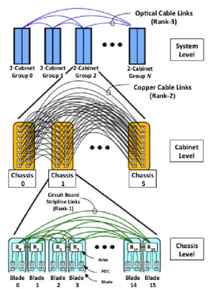
The National Energy Research Scientific Computing Center (NERSC) provides large-scale HPC machines for running scientific applications [1]. For this study, NERSC’s “Edison” Cray XC30 supercomputer was used. “Edison” was named after U.S. inventor and businessman Thomas Alva Edison and has 5,586 computes nodes, 134,064 cores in total. There are 30 cabinets and each cabinet has 3 chassis, each chassis has 16 compute blades, and each compute blade has 4 dual socket nodes. Hence, each cabinet consists of 192 compute nodes. Cabinets are interconnected using Cray’s Aries interconnect withDragonfly topology with 2 cabinets in a single group. Routers

are connected to other routers in the chassis via a backplane. Chassis are connected together to form a two-cabinet group (a total of 6 chassis) using copper cables. Network connections outside the cabinet group require a global link. Optical cables are used for all global links. All two-cabinet groups are directly connected to each other with these optical cables. See Figure 1.2 [1] for the interconnection network on “Edison”. Each compute node has 64 GB of 1866 MHz DDR3 memory (four 8 GB DIMMs per socket) and two 2.4 GHz Intel Xeon E5-2695v2 processors for a total of 24 processor cores, see Figure 1.3[1].

Cache memory, also called CPU memory, is high-speed static random access memory (SRAM) that can be accessed much faster than the regular random access memory (RAM) but is expensive. Traditionally, the cache memory is categorized as “levels” that describe its closeness and accessibil-ity to the core process. This memory is typically integrated directly into the core chip or placed on a separate chip that has a separate bus interconnect with the core. The purpose of cache memory is to store program instructions and data that are used repeatedly in the program. The core process can access this information quickly from the cache rather than having to get it from the shared memory. Fast access to these instructions and data increases the overall speed of the program. On “Edison” each core has its own L1 and L2 caches, with 64 KB (32 KB instruction cache, 32 KB data) and 256 KB, respectively. A 30-MB L3 cache is shared between 12 cores on each processor. Figure1.4[1] shows more details, such as cache memory structure of a compute node on “Edison”. See [1] for more detailed discussions on the configuration of “Edison” and other systems.

HPC is a critical technology since it allows applications to use many processes during execu-tion so that answers are available quickly. For example, financial organizaexecu-tions and investment companies require HPC machines for high speed trading and for running complex simulations for stock and bond trading. To be successful, these organizations try to have answers before their competitors have them. Aerospace companies use HPC machines for designing planes, rockets and jet engines. Car manufactures use HPC for crash test simulations, car design, and engine design. Research at universities and government laboratories use HPC machines extensively.

Figure 1.2: The Dragonfly topology for the interconnection network for NERSC’s “Edison” Cray XC30. Image courtesy of NERSC [1].

To use HPC machines, applications must be written to using parallel programming techniques. Typically, this means using SHared MEMory (SHMEM), the Message Passing Interface (MPI) and/or Open Multi-Processing (OpenMP) and using the Fortran or C/C++ programming lan-guages. OpenMP is used for parallelization of shared memory computers and MPI for parallelization of distributed (and shared) memory computers. Since memory is shared on a node, one can paral-lelize with OpenMP within nodes and MPI between nodes. One could specify 1 MPI process per node and use number of cores/node OpenMP threads to parallelize within a node. However, since

Figure 1.3: The topology of a compute node for NERSC’s “Edison” Cray XC30. Image courtesy of NERSC [1].

there are two processors/sockets per node and since each processor has memory physically close to it, it is generally recommended to use 2 MPI processes per node and use number of cores/pro-cessor OpenMP threads. OpenMP parallelization requires the insertion of directives/pragmas into a program and then compiled with the special compiler option for these directives/pragmas. One can increase performance of an HPC machine by adding accelerators, e.g., Graphical Processing Units (GPUs). To write programs for GPUs one must use Compute Unified Device Architecture (CUDA), CUDA Fortran or use Open Accelerators (OpenACC) with Fortran or C. CUDA is an ex-tension of the C programming language and was created by Nvidia. OpenACC is a directive-based programming model like OpenMP developed by Cray, CAPS, Nvidia and PGI. Like OpenMP 4.0 and newer, OpenACC can be used on both the CPU and GPU architectures.

Figure 1.4: Detailed hierarc hical m ap for the top ology of a compute no de for NERSC’s “Edison” Cra y X C30. Image courtesy of NERSC [ 1 ].

1.1.1.1 One-sided communication

One-sided communication, also known as Remote Memory Access (RMA), is often used in areas such as bioinformatics, computational physics, and computational chemistry to achieve greater per-formance. In 1993 Cray introduced their SHared MEMory (SHMEM) library for parallelization on their Cray T3D, which had hardware support for Remote Direct Memory Access (RDMA) opera-tions. The SHMEM library consists of the one-sided SHMEMget andputoperations, atomic update operations, synchronization routines and the broadcast,collect,reduction andalltoall collective op-erations. In 1994 Message Passing Interface (MPI) 1.0 was introduced. It defined point-to-point and collective operations but did not include one-sided routines. In 1998 the one-sided MPI rou-tines, also known as RMA rourou-tines, were introduced with MPI-2 [2]. MPI-2’s conservative memory model limited its ability to efficiently utilize hardware capabilities, such as cache-coherency and RDMA operations.

In 2012 MPI-3 [3] extended the RMA interface to include new features to improve the usability, versatility and performance potential of MPI RMA one-sided routines. The Cray XC30 supports MPI-3 and utilizes its Distributed Memory Applications (DMAPP) communication library in their implementation of the MPI-3 one-sided routines. From the programmer’s point of view, the differ-ence between SHMEM and MPI one-sided routines is that the SHMEM one-sided routines require remotely accessible objects to be located in the ‘symmetric memory’, which excludes stack mem-ory, while the MPI one-sided routines can access any data on a remote process. However, the MPI one-sided operations require the creation of a special ‘window’ and use of special synchronization routines. More details on MPI and SHMEM one-sided communication are presented below.

The RMA interface in MPI allows one process to specify all communication parameters, both for the ‘sending’ side and for the ‘receiving’ side. The one-sided MPI communications perform RMA operations. MPI must be informed what parts of a ‘process’ memory will be used with RMA operations and which other processes may access that memory. A window object identi-fies the memory and processes that one-sided operations may act on. MPI-3 provides four dif-ferent types of windows: mpi win create (traditional windows), mpi win allocate (allocated

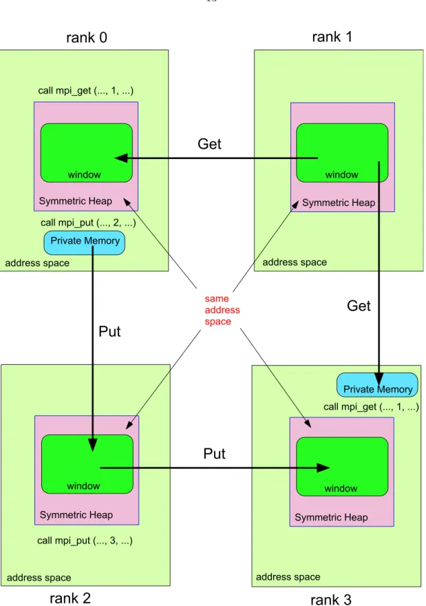
win-dows), mpi win create dynamic (dynamic windows) and mpi win allocate shared (shared memory windows). The traditional windows expose existing memory to remote processes. Each process can specify an arbitrary local base address for the window and all remote accesses are relative to this address. The allocated windows differ from the traditional windows in that the user does not pass allocated memory. The allocated windows allow the MPI library to allocate symmetric window memory, where the base addresses on all processes are the same. By allocating memory instead of allowing the user to pass in an arbitrary local base address, this call can improve the performance for systems which support RMA operations. For this study, the window identifying the memory is created with a call to the new MPI-3 function, mpi win allocate with ‘same size’ ‘info’ key set to true. The ‘info’ argument provides optimization hints to the runtime about the usage of the window. When ‘same size’ is set to true, the implementation may assume that the argument size is identical on all processes. Mpi win allocate is a collective call executed by all processes in the group and it returns the window object that can be used by these processes to perform RMA operations. The memory contained in the window can be accessed by MPI get and put functions, mpi get andmpi put. Mpi get function retrieves data from remote memory into local memory andmpi put moves data from local memory to remote memory. Figure 1.5illustrates the data movement when using MPI get and put operations. The green rectangle represents the window containing the memory to be accessed on each process and the pink square represents the symmetric memory region. Each process has also its private memory which can only be accessed by the process itself represented by a blue rectangle. The window containing the memory to be accessed on each process is created in the symmetric region usingmpi win allocate function and exposes its memory to RMA operations by other processes in a communicator. When using an MPIput operation, a process can ‘put’ data from its window memory or from its private local memory into a remote ‘process’ window. When using an MPIget operation, a process can ‘get’ data from the window of a remote process into its window memory or into its private local memory. Both the rank and position of the memory location can be specified when using MPIget andput functions so that individual elements can be

accessed. These data movement operations are non-blocking and subsequent synchronization on window object is needed to ensure an operation has completed.

MPI provides three synchronization mechanisms: fence, post-start-complete-wait, and lock-unlock. Figure 1.6 illustrates the use of MPI get and put operations, mpi get and mpi put. For ease of exposition, we assume the one-sided communication is between rank i, rank j and rankk processes, where i 6= j 6= k. In our study we used fence and lock-unlock synchronizations. The first call tompi win fenceis required to begin the synchronization epoch for RMA operations. The next call tompi win fence completes the one-sided operations issued by this process as well as the operations targeted at this process by other processes, see Figure1.6a. In thelock-unlock synchro-nization method, the origin process callsmpi win lock to obtain either shared or exclusive access to the window on the target, as shown in Figure 1.6c. After issuing the one-sided operations, it calls mpi win unlock. The target does not make any synchronization call. Whenmpi win unlockreturns, the one-sided operations are guaranteed to be completed at the origin and the target. Mpi win lock is not required to block until the lock is acquired, except when the origin and target are one and the same process. Mpi win free is a collective call executed by all processes in the group that frees the window object and returns a null handle. The memory associated with windows created by a call to mpi win create may be freed after the call returns. If the window was created with mpi win allocate,mpi win free will free the window memory that was allocated inmpi win allocate. This can be called by a process only after it has completed its RMA operations, e.g. the process has called mpi win fence for fence synchronization or mpi win unlock for lock-unlock synchronization. Mpi win free requires a barrier synchronization with an exception to this rule if setting ‘no locks’ ‘info’ key to true when creating the window. In this case, an MPI implementation may free the local window without barrier synchronization.

The SHMEM library provides inter-process communication using one-sided communication, e.g., get and put library calls. Data objects can be stored in a private local memory address or in a remotely accessible memory address space. Objects in the private address space can only be accessed by the processing element (PE) itself and these data objects cannot be accessed by other

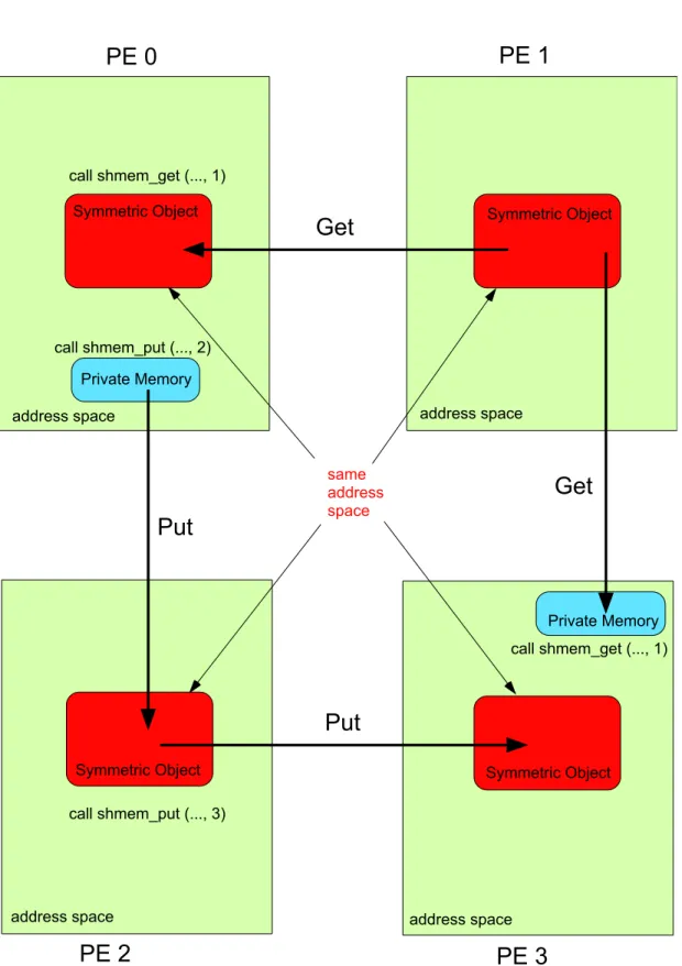
PEs via SHMEM routines. Remotely accessible objects, however, can be accessed by remote PEs using SHMEM routines. Remotely accessible data objects are also known as symmetric objects. Symmetric objects have the same size, type and relative address on all other PEs. Examples of symmetric objects are local static and global variables in C and C++ and variables in common blocks as well as variables with a SAVE attribute in Fortran. Special SHMEM routines allow creation of dynamically allocated symmetric objects. These objects are created in a special memory region called the symmetric heap, which is created during execution at locations determined by the implementation. Symmetric data objects are dynamically allocated in C and C++ using the SHMEM call shmalloc and in Fortran using the SHMEM call shpalloc. Each PE is able to access symmetric variables (Global Address Space), but each PE has its own view of symmetric variables (Partitioned Global Address Space). See Figure 1.7 for an example of how Symmetric Memory Objects may be arranged in memory. The pink square represents the symmetric heap memory region and the red rectangle represents a symmetric object. The private memory which can only be accessed by the PE itself is represented by a blue rectangle.

Figure 1.8 illustrates the data movement when using SHMEM get and put operations and is similar to the Figure 1.5 for MPI. In Figure 1.8 a symmetric object is created statically on the stack or allocated dynamically in the symmetric heap region as described above. Similarly to MPI, when using a SHMEM put operation, a PE can ‘put’ data from its remotely accessible memory or from its private local memory into a symmetric object on a remote PE. When using a SHMEMget operation, a PE can ‘get’ data from a symmetric object of a remote PE into its remotely accessible memory or into its private local memory.

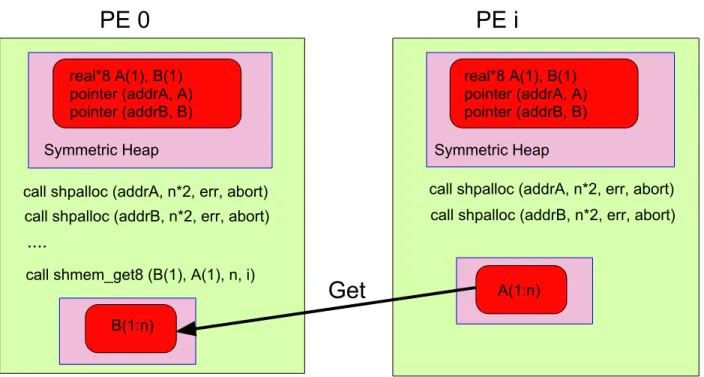
Figures 1.9 and 1.10 illustrate the use of SHMEM get and put operations, shmem get and shmem put. For ease of exposition, we assume the one-sided communication is between PE 0 and PE i, where i is not equal to 0. Both the PE number and position of the memory location need to be specified when using SHMEM get and put functions so that individual elements can be accessed. The shmem get operation is blocking but the shmem put operation is non-blocking making program development more challenging when usingshmem put. As seen in Figure1.9, there

is no need for a synchronization between PE 0 and PE i when using shmem get routine because shmem get routines return when the data has been copied from the remote PE into the local PE. However, if the program on PE i may need to change A, then PE i needs to know when PE 0 has copied A from its memory so that it is safe to change A. In this case synchronization between the two processes: PE 0 and PE i is needed and should be done in a similar manner as shown for shmem put by using shmem fence withshmem wait until presented below.

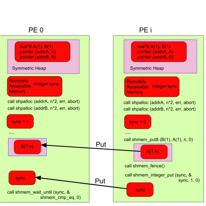
Figure1.10illustrates how PEi ‘puts’ the data on PE 0. Sinceshmem put routines return when the data has been copied out of thelocal PE, but not necessarily before the data has been delivered to the remote data object, subsequent synchronization is needed to ensure the put operation has completed. Synchronization between PE i and PE 0 is achieved by calling the library functions shmem fence andshmem wait until. Theshmem fence routine insures that all priorput operations issued to a particular destination PE are written to the symmetric memory of that destination PE, before any followingput operations to that samedestination PE are written to the symmetric memory of that destination PE. PEi issues a shmem fence after issuing a shmem put on process 0 and then issues a shmem integer put of a synchronization variable, sync, on PE 0. PE 0 waits for the sync variable to be updated to 0 by the PEi (the sender PE) by issuingshmem wait until. After the shmem wait until returns, it is safe to use the array B on PE 0 with values from the remote put operation issued by PE i. Comparing Figure 1.9 with Figure 1.10 one can see that using shmem put routine is more challenging than using shmem get routine since it requires the use of a synchronization variable, sync, in addition to the shmem fence routine. For applications where global synchronization is required, synchronization is achieved by calling the library function shmem barrier all.

rank 0

rank 1

rank 2

rank 3

Get

Put

Get

Put

Symmetric Heap Symmetric Heap

Symmetric Heap _{Symmetric Heap}

window window

window _window

address space

address space address space

same address space call mpi_get (..., 1, ...) call mpi_get (..., 1, ...) call mpi_put (..., 2, ...) call mpi_put (..., 3, ...) Private Memory Private Memory

Figure 1.5: A schematic diagram of remote memory access using a window object created with mpi win allocate for MPIget and put.

Process i

Process j

MPI_Win_fence (win)

MPI_Put (j)

MPI_Get (j)

MPI_Win_fence (win)

MPI_Win_fence (win)

MPI_Put (i)

MPI_Get (i)

MPI_Win_fence (win)

(a) Fence synchronization

Process i MPI_Win_start (j) MPI_Put (j) MPI_Get (j) MPI_Win_complete (j) Process k MPI_Win_start (j) MPI_Put (j) MPI_Get (j) MPI_Win_complete (j) Process j MPI_Win_post (i, k) MPI_Win_wait (i, k) (b) Post-start-complete-wait synchronization Process i MPI_Win_allocate (win) MPI_Win_lock (shared, j) MPI_Put (j) MPI_Get (j) MPI_Win_unlock (j) MPI_Win_free (win) Process j MPI_Win_allocate (win) MPI_Win_free (win) Process k MPI_Win_allocate (win) MPI_Win_lock (shared, j) MPI_Put (j) MPI_Get (j) MPI_Win_unlock (j) MPI_Win_free (win) (c) Lock-unlock synchronization

Figure 1.6: The three synchronization mechanisms for one-sided communication in MPI. The ar-guments indicate the target rank, wherei6=j 6=k.

PE 0

PE 1

Private Memory Private Memory

Remotely Accessible Memory Remotely Accessible Memory address space Symmetric Heap same address space integer x real*8 y

PE 0

PE 1

PE 2

PE 3

Get

Put

Get

Put

address space _{address space}

same address space

Symmetric Object

Symmetric Object _{Symmetric Object}

call shmem_get (..., 1) call shmem_get (..., 1) call shmem_put (..., 2) call shmem_put (..., 3) Private Memory Private Memory

Figure 1.8: A schematic diagram of remote memory access using a symmetric object for SHMEM get and put.

PE 0

PE i

pointer (addrA, A) pointer (addrB, B) Symmetric Heap

call shmem_get8 (B(1), A(1), n, i)

....

Symmetric Heap

call shpalloc (addrB, n*2, err, abort)

call shpalloc (addrA, n*2, err, abort)

B(1:n) A(1:n) real*8 A(1), B(1) pointer (addrA, A) pointer (addrB, B)

Get

call shpalloc (addrB, n*2, err, abort)

PE 0

PE i

pointer (addrA, A) pointer (addrB, B) Symmetric Heap

call shpalloc (addrA, n*2, err, abort)

call shmem_wait_until (sync, & shmem_cmp_eq, 0)

....

call shpalloc (addrB, n*2, err, abort)

call shpalloc (addrA, n*2, err, abort) call shpalloc (addrB, n*2, err, abort)

....

Accessible Memory

integer sync Remotely

Accessible Memory

integer sync

call shmem_put8 (B(1), A(1), n, 0)

call shmem_fence()

call shmem_integer_put (sync, & sync, 1, 0) sync sync sync = 1 sync = 0 B(1:n) A(1:n)

Put

Put

1.1.1.2 HPC workflow optimization

A simple definition of a workflow is the repetition of a series of activities or tasks that are necessary to obtain a result. The HPC workflow can be defined as the flow of tasks that need to be executed to compute on HPC machines and process the results. Tasks within the HPC workflow can be jobs that run on HPC resources or auxiliary assignments that run outside of HPC resources. Example tasks include writing scripts and configuration files, uploading the input files (input data, source codes, scripts and configuration files) to an HPC machine, submitting a job and performing an analysis. Figure1.11 shows a typical example for the HPC workflow diagram.

The HPC workflows are a means by which scientists can model their analysis. With the evolution of HPC systems, it important to facilitate scientists to be able to easily rerun their analysis on both existing and new HPC computers. Tools are designed to optimize the HPC workflow. An HPC workflow optimization tool offers functionality in several areas: workflow orchestration, HPC machine provisioning, job submission and data analysis.

To orchestrate these tasks, the tool uses a workbench with task execution engine, such as the Cyclone Database Implementation Workbench (CyDIW) developed at Iowa State University [4,5]. For HPC machine provisioning, the tool writes the configuration files, which match the size and characteristics of an HPC machine to the HPC workflow. The tool also writes the scripts needed for the job submission and it provides access to HPC resources through job schedulers. These schedulers add jobs to a queue until processors and memory become available. Next, the tool suspends execution and waits for the job to finish. Once the job is completed, it collects the output data, copies the data to the local machine and performs the data analysis, such as generating tables and graphs for visualization.

To conclude, an HPC workflow optimization tool will automatically write appropriate config-uration files and scripts and submit them to the job scheduler, collect the output data for each application and then perform a data analysis, such as generating various tables and graphs.

In this work, we implemented the HPC–Bench tool using CyDIW, which optimizes the HPC benchmarking workflow and saves time in analyzing performance results by automatically generat-ing performance graphs and tables.

prepare source codes write scripts and

configuration files

copy the input files to the HPC machine

submit the scripts to the job scheduler

Process 0 application 1 ... application n Process 1 application 1 ... application n Process p-1 application 1 ... application n

...

copy the output files to the local machine

process the output files to generate

tables and graphs

share the results

1.1.2 Machine Learning

Professor Andrew Ng from Stanford University gives a nice introduction to machine learning along with its applications in the “Machine Learning” online open course [6]. Following is a sum-mary of his introduction.

Machine learning is one of the most exciting fields of computing today and has become a part of everyday life. We are using machine learning many times a day without even knowing it. For example, web searching engines, such as Google and Bing use machine learning software to rank pages. When a photo application recognizes people in the pictures, that’s also machine learning. Another example is an email anti-spam filter, which has learned to distinguish spam from non-spam emails. The recommendations for the books we buy, the movies we watch, the music we listen to, the sports we follow, the driving directions we need are also driven by machine learning algorithms. Machine learning is a field that had grown out of the field of artificial intelligence (AI). AI is used to build intelligent machines, however, there are just a few basic things that one could program a machine to do, such as finding the shortest path from A to B. People don’t know how to write AI programs for web searching or photo tagging or email anti-spam. The only way to do these things is to have a machine learn to do it by itself.

Let us try to answer the following question: “What is machine learning?”. Arthur Samuel defined machine learning as “the field of study that gives computers the ability to learn without being explicitly programmed.” In 1950 Samuel wrote a checkers playing program by programming tens of thousands of games against himself. By watching what sorts of board positions tended to lead to wins and what sort of board positions tended to lead to losses, the checkers playing program learned over time what are good board positions and what are bad board positions. Eventually, it learned to play checkers better than Arthur Samuel. Because a computer has the patience to play tens of thousands of games, it was able to get more checkers playing experience than a human. Tom Mitchell provides a more modern definition of machine learning: “A computer program is said to learn from experience E with respect to some class of tasks T and performance measure P, if its performance at tasks in T, as measured by P, improves with experience E.” Taking the example

above of playing checkers, E is the experience of playing many games of checkers, T is the task of playing checkers, andP is the probability that the program will win the next game.

Autonomous vehicles or helicopters are similar examples of machine learning applications. There are no AI computer programs to make a helicopter fly by itself or a car drive by itself. The solution is having a computer learn by itself how to fly the helicopter or drive the car. Actually, most of computer vision today is applied machine learning, e.g., autonomous robotics, handwriting recognition and natural language processing.

In recent years, machine learning touched many domains of industry and science. One of the reasons machine learning has grown in popularity lately is the growth of data and, along with that, the growth of automation. One application of machine learning in industry is database mining. Many Silicon Valley companies are collecting web click data or clickstream data and are trying to use machine learning algorithms to mine this data to understand the users in order to serve them better. All fields of science have larger and larger datasets that can be understood using machine learning algorithms. For example, machine learning uses electronic medical records data and turn it into knowledge, which enables one to understand diseases better. It is worthy mentioning the application of machine learning in computational biology as well. With automation, biologists are collecting lots of data about gene sequences, DNA sequences, etc. Machine learning algorithms use this data to provide a better understanding of the human genome, and what it means to be human. The AI dream is to build truly intelligent machines, i.e., as intelligent as humans. For example, build robots that tidy up the house. First have the robot watch a human demonstrate the task and then learn from that. The robot will watch what objects the human picks up and where the human puts them and then try to do the same thing by itself. We’re a long way away from that goal, but many scientists think the best way to make progress on this is through learning algorithms, inspired by the structure and function of the human brain, called artificial neural networks. More details are provided below.

1.1.2.1 Artificial neural networks

Dr. Robert Hecht-Nielsen defined an artificial neural network (ANN) as “a computing system made up of a number of simple, highly interconnected processing elements, which process informa-tion by their dynamic state response to external inputs” [7]. ANNs were inspired by the structure and function of the human brain with complex tasks, such as learning, memorizing and generalizing. ANNs started to be very widely used throughout the 1980’s and 1990’s, but their popularity diminished in the late 1990’s. However, with the advancement of computers and better algorithms, ANNs have had a major resurgence in the last decade. Today they are known as the state-of-the-art technique for many applications.

ANNs are typically organized in layers. This arrangement gives a class of ANN called multi-layer ANN. ANNs are composed of an input multi-layer, one or more hidden multi-layers and an output multi-layer. Layers are made up of a number of highly interconnected processing units, called artificial neurons (ANs). The ANs contain an activation function and are connected with each other via adaptive synaptic weights. The AN collects all the input signals and calculates anet signal as the weighted sum of all input signals. Next, the AN calculates and transmits an output signal by applying the activation function to thenet signal. Input data are presented to the network via the input layer, which communicates to one or more hidden layers, where the actual processing is done via the weighted connections. The hidden layers then link to the output layer, which gives the results. The type of ANN, which propagates the input through all the layers and has no feed-back loops is called afeed-forward multi-layer ANN, see Figure1.12. For this study, we adopt and work with a feed-forward three-layer ANN.

For function approximation, a sigmoid orsigmoid–like andlinear activation functions are usu-ally used for the neurons in the hidden and output layer, respectively.

The development of an ANN is a two-step process with training and testing stages. In the training stage, the ANN adjusts its weights until an acceptable error level between desired and predicted outputs is obtained. The difference between desired and predicted outputs is measured

Figure 1.12: An example of a feed-forward multi-layer ANN [8].

by the error function, also called the performance function. A common choice for the error function ismean square error (MSE).

There are various training algorithms for feed-forward ANNs. The training algorithms use the gradient of the error function to determine how to adjust the weights to minimize the error function. The gradient is determined using a technique calledback-propagation[9], which involves performing computations backwards through the network. Theback-propagation computation is derived using the chain rule of calculus.

The back-propagation algorithm minimizes the error function as a function of the weights. The error surface is a hyperparaboloid in the weights’ vector space, but it is rarely ‘smooth’. There are many variations of the back-propagation algorithm. The simplest implementation of back-propagation learning updates the network’s weights in the direction in which the error function decreases most rapidly, i.e., the negative of the gradient. This is known as the gradient descent method. For example, for the first hidden layer, one iteration of this algorithm can be written as:

wn+1 =wn+β×δn×x, (1.1)

where wn is the vector of current weights associated with the input connection links, δn is the current gradient, β is the learning rate, andx is the vector of input signals. See Figure1.13 for a

schematic representation for the weights’ update associated with the input connections of a given neuron. Learning rate controls the change in the weight from one iteration to another. As a general rule, smaller learning rates are considered as stable but cause slower learning. On the other hand, higher learning rates can be unstable causing oscillations and numerical errors but speed up the learning.

Figure 1.13: Weights’ update using the back-propagation algorithm [8].

Figure1.14shows the gradient descent implementation of theback-propagationalgorithm which goes towards the global minimum along the steepest vector of the error surface. The global minimum is the theoretical solution with the lowest possible error. In most problems, the solution space is quite irregular with several local minima, which can cause the algorithm to find a local minimum instead of the global minimum. Since the nature of the error space can not be known a priori, many individual runs of the training algorithm are needed to determine the best solution. Furthermore, since the training of the network depends on the initial starting solution, it is important to train the network several times using different starting points.

The gradient descent with momentum implementation of the back-propagation algorithm pro-vides inertia to escape local minima. The idea of gradient descent with momentum is to simply add a certain fraction of the previous weight update to the current one, to avoid being stuck in local minima. This fraction represents the momentum rate parameter. Equation1.1 becomes:

wn+1 =wn+β×δn×x+α×(wn−wn−1), (1.2)

whereα is the momentum rate.

Figure 1.14: The gradient descentback-propagationalgorithm updates the network’s weights in the direction of the negative gradient of the error function [8].

There are two different ways in which the gradient descent algorithm can be implemented: incremental mode and batch mode. In the incremental mode, the gradient is computed and the weights are updated after each input is applied to the network. In the batch mode all of the inputs are applied to the network before the weights are updated. Theback-propagationtraining algorithm in batch mode performs the following steps:

• Select a network architecture.

• Initialize the weights to small random values.

• Present the network with all the training examples from training set.

• Forward pass: compute the net activations and outputs of each neuron in the network with the current value of the weights.

• Backward pass: compute the errors for each neuron in the network.

• Update weights as a function of the back-propagated errors, e.g., Equations 1.1and 1.2.

• If the stopping criterion is satisfied, then stop: – maximum number of epochs

– a minimum value of the error function evaluated for the training data set – the over–fitting point

The gradient descent and gradient descent with momentum algorithms are too slow for prac-tical problems. There are several high performance algorithms, which operate in the batch mode, that can converge from ten to one hundred times faster than than gradient descent algorithms. Heuristic techniques were developed from an analysis of the performance of the standard steepest descent algorithm, such as variable learning rate back-propagation and resilient back-propagation. Some standard numerical optimization techniques are: conjugate gradient, quasi-Newton [10] and Levenberg-Marquardt [9,11]. For this study, Levenberg-Marquardt algorithm was used along with Bayesian regularization of David MacKay [12] to improve ANN performance.

Once an ANN is trained, it can be used as an analytical tool on new data that were not used in the training process. This is the testing stage of the ANN. The predicted output from the new input data can then be used for further analysis and interpretation. For further and general background on the ANN refer to [13,14].

1.1.3 Nuclear Physics

Before describing the models of nuclear structure, it is useful to make a short comparison of the characteristics of atoms and nuclei. The nuclear structure is more complex than the atomic structure. Atoms have a center of attraction for all the electrons and inter-electronic forces generally play a small role. The predominant force (Coulomb) is well understood. Nuclei, on the other hand, have no center of attraction. A nucleus is made up of positively charged protons and neutral (no charge) neutrons, which are called nucleons. The nucleons are held together by their inter-nucleon interactions which are much more complicated than Coulomb interactions. There is a very strong and short-range (∼1 f mor 1×10−15 meters) force that pulls nucleons toward each other, and an even stronger repulsive force at even shorter distances that keeps them from overlapping each other. This is why a nucleus, in a classical sense, may be viewed as a closely packed set of spheres that are almost touching one another as seen in example from Figure 1.15for7Li [15]. Natural lithium is made up of two isotopes: 7Li (92.5%) and6Li (7.5%). In this work, we studied the ground state (gs) energy and proton root-mean-square (rms) radius of6Li, which has 3 protons and 3 neutrons, and a mass number of 6.

Figure 1.15: Schematic diagram of the 7Li nucleus, which has 3 protons and 4 neutrons, giving it a total mass number of 7 [15].

Furthermore, all atomic electrons are alike, whereas there are two species of nucleons: protons and neutrons. This allows a richer variety of structures for nuclei than for atoms. Notice that there are approximately 100 types of atoms, but an estimated 7,000 nuclei produced in nature. Neither atomic nor nuclear structures can be understood without quantum mechanics which significantly enhances the computational complexity.

Many models were proposed to study the nuclear structure and reactions. Liquid Drop Model was the first model proposed by George Gamow. According to this model, the atomic nucleus behaves like the molecules in a drop of liquid. This model does not explain all the properties of the nucleus, but describes very well the nuclear binding energies. Based on Liquid Drop Model, the nuclear binding energy was given as a function of the mass number A and the number of protons Z. This represents the Weizs¨acker formula, also called the semi-empirical mass formula, that was published in 1935 by German physicist Carl Friedrich von Weizs¨acker.

Later came the Nuclear Shell Model which was first proposed in 1948 by Maria Goeppert-Mayer, the second woman to win a Nobel Prize in physics, after Marie Curie. The Nuclear Shell Model deals with the features of energy levels. A shell is the energy level where particles of same energy can reside. The Nuclear Shell Model describes the arrangement of the nucleons in the different shells of the nuclei. For general background on nuclear physics, see [16,17,18].

In the Nuclear Shell Model, a nucleus consisting of A-nucleons withN neutrons and Z protons (A =N+Z) is described by the quantum Hamiltonian with kinetic energy (Trel) and interaction

(V) terms HA=Trel+V = 1 A X i<j (~pi−~pj)2 2m + A X i<j Vij+ A X i<j<k Vijk+ . . . . (1.3)

Here, m is the nucleon mass (taken as the average of the neutron and proton mass), ~pi is the momentum of thei-th nucleon,Vij is the nucleon-nucleon (NN) interaction including the Coulomb interaction between protons,Vijk is the three-nucleon interaction and the interaction sums run over

all pairs and triplets of nucleons, respectively. Higher-body (up to A-body) interactions are also allowed and signified by the three dots.

One can not solve the nuclear quantum many-body problem exactly or accurately describe nuclear structure even when good precision is achieved for the lightest nuclei. One main limitation, which actually motivates computational nuclear structure investigations, arises because the NN interaction is not known precisely from the underlying theory of the strong interaction, called Quantum Chromodynamics (QCD). However, there have been successful attempts to evaluate the NN interaction in the last two decades. The NN interaction was derived as a realistic interaction that fulfills the symmetries required by QCD and describes well the properties of light nuclei, e.g., Daejeon16 [19]. When interactions that describe NN scattering data with high accuracy are employed, the approach is considered to be a first principles or ab initio method. No-Core Shell Model (NCSM) [20] is anab initio approach in which all nucleons are dynamically involved in the interaction and are treated on an equal footing.

The NCSM casts the non-relativistic quantum many-body problem as a finite Hamiltonian matrix eigenvalue problem expressed in a chosen, but truncated, basis space. A popular choice of basis representation is the three-dimensional harmonic-oscillator (HO) basis that we employ in this work. The HO basis is characterized by two parameters: the HO energy, ¯hΩ, and the many-body basis space cutoff,Nmax.

The first parameter, ¯hΩ, is the HO energy, and represents the spacing between major shells. Each shell is labeled uniquely by the HO quanta of its orbits, N = 2n+l (n and l are the radial and orbital angular momentum quantum numbers, respectively), which begins with 0 for the lowest shell and increments in steps of unity. Orbits are specified by the set of quantum numbers nljmj, wherej is the total angular momentum quantum number, and mj is the total angular momentum projection along the z-axis quantum number. Due to the spin-orbit (SO) interaction, the energies of states of the same orbital angular momentum, l, but with differentj can not be identical. This arises from the fact that when the orbital angular momentum vector is parallel to the spin vector, the SO interaction energy is attractive. In this case, j = l+s = l+ 1/2, where s is the spin

quantum number. When the orbital angular momentum vector is opposite to the spin vector, the SO interaction energy is repulsive. In this case, j = l−s = l−1/2. Moreover, each unique arrangement of fermions (neutrons and protons) within the available HO orbits must satisfy the Pauli principle. The Pauli principle states that the number of nucleons (fermions) needed to fill each orbital is 2, similar to the electrons in atomic orbitals. Hence, according to the Pauli principle a maximum of two neutrons or protons are allowed into each orbital.

Let us take 6Li to illustrate an example of shell model filling. First, place the three protons into the lowest available orbitals. The protons in the 0s1/2 state must be paired according to

the Pauli principle. This results in the following configuration for the protons: (0s_1/2)2_(0p 3/2)1.

Similarly, place the three neutrons into their lowest available orbitals. The neutron configuration is: (0s1/2)2(0p3/2)1.

The second parameter, Nmax, is the many-body basis space cutoff. Nmax is defined as the

maximum number of the total HO quanta allowed in the many-body basis space above the minimum HO configuration for the specific nucleus needed to satisfy the Pauli principle. Its use allows one to preserve Galilean invariance–to factorize all eigenfunctions solutions into a product of intrinsic and center-of-mass motion (CM) components. Because Nmax is the maximum of the total HO quanta

above the minimal HO configuration, it is possible to have at most one nucleon in the highest HO single-particle state consistent withNmax.

Figure1.16shows an example for the proton (right) and neutron (left) energy level distributions in6_{Li, where one unit HO quanta,N, is one unit of quantity (2n+l). The unperturbed gs (the HO}

configuration with the minimum HO energy) is defined to be the Nmax = 0 configuration, shown

as Min(Nmax) = 0. Note, the configuration shown in Figure 1.16 has four excitation HO quanta

for neutrons and two excitation HO quanta for protons above the minimum configuration. This is referred to as “Nmax = 6” configuration or “6¯hΩ” configuration in the ab initio NCSM. The

remaining states allowed with an Nmax = 6 cutoff consist of all possible arrangements of the six

to many-body basis states with total many-body HO quanta, Ntot =

A X i=1

Ni ≤N0+Nmax, where N0 is the minimal number of quanta for that nucleus, which is 2 for 6Li.

Figure 1.16: 6Li proton and neutron energy level distributions in NCSM atNmax= 6 using an HO

potential.

Each unique arrangement of fermions (neutrons and protons) within the available HO orbits, consistent with the Pauli principle, constitutes a many-body HO basis state. The many-body HO basis states are employed to evaluate the Hamiltonian, H. Nmax limits the total number of HO

quanta allowed in the many-body basis states and, thus, limits the dimension,D, of the Hamiltonian matrix in that basis space. These Hamiltonian matrices are sparse, the number of non-vanishing matrix elements follows an approximate scaling rule ofD3/2. For these large and sparse Hamiltonian matrices, the Lanczos method is one possible choice to find the extreme eigenvalues [21]. Usually, the basis includes either only many-body states with even values of Ntot (and respectively Nmax),

which correspond to states with the same (positive for6Li) parity as the unperturbed gs, and are called the “natural” parity states, or only with odd values of Ntot (and respectivelyNmax), which

correspond to states with “unnatural” (negative for6Li) parity.

The ab initio NCSM calculations are performed with the MFDn code [22, 23, 24], a hybrid MPI/OpenMP code for ab initio nuclear structure calculations. Due to the strong short-range correlations of nucleons in a nucleus, a large basis space is required to achieve convergence in this 2-dimensional parameter space (¯hΩ, Nmax), where convergence is defined as independence of both

parameters within evaluated uncertainties. The requirement to simulate the exponential tail of a quantum bound state with HO wave functions possessing Gaussian tails places additional demands on the size of the basis space. However, one faces major challenges to approach convergence since, as the size of the space increases, the demands on computational resources grow rapidly. To obtain the nuclear observables as close as possible to the exact results, one seeks solutions in the largest feasible basis spaces. These results are then used in attempts to extrapolate to the infinite basis space using various extrapolation techniques [25,26,27].

Using such extrapolation methods, one investigates the convergence pattern with increasing basis space dimensions and thus obtains, to within quantifiable uncertainties, results corresponding to the complete basis. In this work, we implement a feed-forward artificial neural network (ANN) method as an extrapolation tool to obtain results along with their extrapolation uncertainties and compare with results from other extrapolation methods.

1.2 Thesis Organization

This thesis presents three papers that have been refereed and accepted for publication and one posted online and submitted for publication. Each paper addresses a different aspect of high per-formance computing (HPC). The first paper (Chapter2) compares the performance and scalability of MPI and SHMEM with emphasis on the one-sided communication routines.

Chapter3presents the HPC–Bench tool, which can be used to optimize HPC workflow. Today’s high performance computers are complex and constantly evolving making it important to be able

to easily evaluate the performance and scalability of parallel applications on both existing and new HPC machines. The evaluation of the performance of applications can be time consuming and tedious. To optimize this process, the authors developed a tool, HPC–Bench, using the Cyclone Database Implementation Workbench (CyDIW) developed at Iowa State University [4, 5]. HPC– Bench integrates the workflow into CyDIW as a plain text file and encapsulates the specified commands for multiple client systems. By clicking the “Run All” button in CyDIW’s graphical user interface (GUI), HPC–Bench will automatically write appropriate scripts and submit them to the job scheduler, automatically collect the output data for each application and then automatically generate performance tables and graphs. Use of HPC–Bench is illustrated with several MPI and SHMEM applications [3], which were run on the National Energy Research Scientific Computing Center’s (NERSC) Edison Cray XC30 HPC computer for different problem sizes and for different number of MPI processes/SHMEM processing elements (PEs) to measure their performance and scalability. Chapter 3 describes the design of HPC–Bench and gives illustrative examples using complex applications [28] on a NERSC’s Cray XC30 HPC machine.

Chapters4and5discuss a novel application of machine learning to a nuclear physics application. Chapter 5is a continuation of the research presented in Chapter 4. A feed-forward ANN method is used as an extrapolation tool to obtain the ground state (gs) energy and the ground state (gs) point-proton root-mean-square (rms) radius. Chapter 5 extends the work presented in Chapter 4 and presents results using multiple datasets, which consist of data through a succession of cutoffs: Nmax= 10,12,14,16 and 18. The work in Ch