Coupled Clustering: A Method for Detecting Structural Correspondence

(1)

Coupled Clustering: A Method for Detecting

Structural Correspondence

Zvika Marx [email protected]

The Interdisciplinary Center for Neural Computation The Hebrew University of Jerusalem

Givat-Ram, Jerusalem 91904, Israel and Department of Computer Science Bar-Ilan University

Ramat-Gan 52900, Israel

Ido Dagan [email protected]

Department of Computer Science Bar-Ilan University

Ramat-Gan 52900, Israel

Joachim M. Buhmann [email protected] Institut für Informatik III

University of Bonn

Römerstr. 164, D-53117 Bonn, Germany

Eli Shamir [email protected]

School of Computer Science and Engineering The Hebrew University of Jerusalem

Givat-Ram, Jerusalem 91904, Israel

Editors: Carla E. Brodley and Andrea Danyluk

Abstract

This paper proposes a new paradigm and a computational framework for revealing equivalencies (analogies) between sub-structures of distinct composite systems that are initially represented by unstructured data sets. For this purpose, we introduce and investigate a variant of traditional data clustering, termed coupled clustering, which outputs a configuration of corresponding subsets of two such representative sets. We apply our method to synthetic as well as textual data. Its achievements in detecting topical correspondences between textual corpora are evaluated through comparison to performance of human experts.

Keywords: Unsupervised learning, Clustering, Structure mapping, Data mining in texts, Natural language processing

1. Introduction

Unsupervised learning methods aim at the analysis of data, based on patterns within the data itself while no supplementary directions are provided. Two extensively studied unsupervised tasks are: (a) assessing similarity between object pairs, typically quantified by a single value denoting an overall similarity level, and (b) detecting, through various techniques, the detailed structure of individual composite objects.

(2)

objects similar. According to the common view, two given objects are considered similar if they share a relatively large subset of common features, which are identifiable independently of the role they perform within the internal organization of the compared objects. Nonetheless, one might wonder how faithfully a single value (or a list of common features) represents the whole richness and subtlety of what could be conceived as similar. Indeed, cognitive studies make a distinction between surface-level similar appearance and deep structure-based correspondence relationships, such as in analogies and metaphors. Motivated by this conception of structure-related similarity, we introduce in this paper a novel conceptual and algorithmic framework for unsupervised identification of structural correspondences.

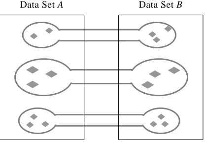
Data clustering techniques—relying themselves on vectorial representations or similarities within the clustered elements—impose elementary structure on a given unstructured corpus of data by partitioning it into disjoint clusters (see Subsection 2.1 for more details). The method that we introduce here—coupled clustering—extends the standard clustering methods for a setting consisting of a pair of distinct data sets. We study the problem of partitioning these given two sets into corresponding subsets, so that every subset is matched with a counterpart in the other data set. Each pair of matched subsets forms jointly a coupled cluster. A resulting configuration of coupled clusters is sketched in Figure 1. A coupled cluster consists of elements that are similar to one another and distinct from elements in other clusters, subject to the context imposed by aligning the clustered data sets with respect to each other. Coupled clustering is intended to reflect comparison-dependent equivalencies rather than overall similarity. It produces interesting results in cases where the two clustered data sets are overall not very similar to each other. In such cases, coupled clustering yields inherently different outcome than standard clustering applied to the union of the two data sets: standard clustering might be inclined to produce clusters that are exclusive to elements of either data set. Coupled clustering, on the other hand, is directed to include representatives from both data sets in every cluster. Coupled clustering is a newly defined computational task of general purpose. Although it is ill posed, similarly to the standard data-clustering problem, it is potentially usable for a variety of applications.

Coupled clustering can potentially be utilized to reveal equivalencies in any type of data that can be represented by unstructured data sets. Representative data sets might contain, for instance, pixels or contours sampled from two image collections, or patterns of physiological measurements collected from distinct populations and so on.

Data Set A Data Set B

(3)

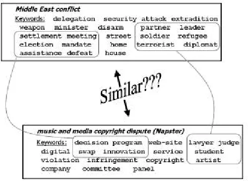
The current work concentrates on textual data, while the variety of other conceivable applications should be investigated within subsequent projects. Specifically, we apply coupled clustering to pairs of textual sources—document collections or corpora— containing information regarding two distinct topics that are characterized by their own terminology and key-concepts. The target is to identify prominent themes, categories or entities, for which a correspondence can be identified simultaneously within both corpora. The keyword sets in Figure 2, for instance, have been extracted from news articles regarding two conflicts of distinct types: the Middle-East conflict and the dispute over copyright of music and other media types (the “Napster case”). The question of whether, and with relation to which aspects, these two conflicts are similar does not seem amenable to an obvious straightforward analysis. Figure 2, however, demonstrates some non-trivial correspondences that have been identified by our method. For example: the role played within the Middle East conflict by individuals—such as ‘soldier’, ‘refugee’, ‘diplomat’—has been aligned by our procedure, in this specific comparison, with the role of other individuals—‘lawyer’, ‘student’ and ‘artist’—in the copyright dispute.

Cognitive research, most notably the structure mapping theory (Gentner, 1983), has emphasized the importance of the various modes of similarity assessment for a variety of mental activities. In particular, the role of structural correspondence is crucial in analogical reasoning, abstraction and creative thinking, involving mental maps between complex domains, which might appear unrelated at first glance. The computational mechanisms introduced for implementing the structure mapping theory and related approaches typically require as input data items that are encoded a priori with structured knowledge (see Section 7 for further discussion). Our framework, in distinction, assumes knowledge of abstracted type, namely similarity values pertaining to unstructured data elements, while the structure that underlies the correspondence between the compared domains emerges through the mapping process itself.

Structural equivalencies consistently enlighten various fields of knowledge and scholarship. Historical situations and events, for instance, provide a rich field for the construction of structural analogies. A unique enterprise dates back to Plutarch's “Parallel Lives”, in which Greek public figures are paired with Roman counterparts

(4)

whose “feature vectors” of life events and actions exhibit structural similarity.1 In comparison to ancient times, the current era presents growing accessibility to large amounts of unstructured information. Indeed, intensive research takes place, within areas such as information retrieval and data mining, aiming at the needs that evolve in an information-intensive environment. This line of research typically addresses similarity in its surface feature-based mode. A subsequent objective would be to relate and compare separate aggregations of information with one another through structure mapping. In the field of competitive intelligence, for example, one attempts to obtain knowledge of the players in a given industry and to understand the strengths and weaknesses of the competitors (Zanasi, 1998). In many cases, plenty of data— financial reports, white papers and so on—are publicly available for any type of analysis. The ability to map automatically knowledge regarding products, staff or financial policy of one company onto the equivalent information of another company could make a valuable tool for inspection of competing firms. If applied appropriately to such readily available data, structure mapping might turn into a useful approach in future information technology.

The current paper extends earlier versions of the coupled clustering framework that have been presented previously (Marx, Dagan and Buhmann, 2001; Marx and Dagan, 2001). In Section 2, we review the computational methods used within our procedure, namely standard clustering methods and co-occurrence based similarity measures. The coupled clustering method is formally introduced in Section 3. Then, we demonstrate our method's capabilities on synthetic data (Section 4) as well as in detecting equivalencies in textual corpora, including elaboration of the conflict example of Figure 2 and identification of corresponding aspects within various religions (Section 5). Evaluation is conducted through comparison of our program's output with clusters that were constructed manually by experts of comparative studies of religions (Section 6). Thereafter, we compare the coupled clustering method with related research (Section 7). In Section 8, we illustrate how coupled clustering, which is essentially a feature-based method, could be used to detect equivalent relational patterns of the type that have been motivating cognitive theories of structural similarity. The paper ends with conclusions and directions for further research (Section 9).

2. Computational Background

The following two subsections address the computational procedures that are utilized within the coupled-clustering framework. The first subsection, reviewing the data-clustering task, concentrates on the relevant details of the particular approach that we have adapted for our algorithm (Subsection 3.3), by Puzicha, Hofmann and Buhmann (2000). The following subsection reviews methods for calculating similarity values. It exemplifies co-occurrence based techniques of similarity assessment, utilized later for generating input for coupled clustering applied to keyword data sets extracted from textual corpora (Sections 5, 6).

2.1. Cost-based Pairwise Clustering

Data clustering methods provide a basic and widely used tool for detecting structure within initially unstructured data. Here we concentrate on the basic clustering task, namely partitioning the given data set into relatively homogenous and well-separated clusters. Hereinafter, we shall refer to this standard task by the term standard

(5)

clustering, to distinguish it from coupled clustering. The notion of data clustering can be extended to include several additional methods, which would not be discussed further here, for instance, methods that output overlapping clusters or hierarchical clustering that recursively partitions the data.

Our motivation for utilizing a clustering mechanism for mapping structure stems from the view of clustering as extracting of meaningful components in the data (Tishby, Pereira and Bialek, 1999). This view is particularly sensible when the clustered data is textual. In this case, clusters of words (Pereira, Tishby and Lee, 1993) or documents (Lee and Seung, 1999; Dhillon and Modha, 2001) can be referred to as explicating prominent semantic categories, topics or themes that are substantial within the analyzed texts.

Clustering often relies on associating data elements with feature vectors. In this case, each cluster can be represented by some averaged (centroid) vectorial extraction (e.g., Pereira, Tishby and Lee, 1993; Slonim and Tishby, 2000b). An alternative approach, pairwise clustering, is based on a pre-given measure of similarity (or distance) between the clustered elements, which are not necessarily embeddable within a vector space or even a metric space. Feature vectors, if not used directly for clustering, can still be utilized for defining and calculating a pairwise similarity measure.

The clustering task is considered ill-posed: there is no pre-determined criterion measuring objectively the quality of any given result. However, there are clustering algorithms that integrate the effect of the input—feature vectors or similarity values— through an objective function, or cost function, which assigns to any given partitioning of the data (clustering configuration) a value denoting its assumed quality.

The clustering method that we use in our work follows a cost-based framework for pairwise clustering recently introduced by Puzicha, Hofmann and Buhmann (2000). They present, analyze and classify a family of clustering cost functions. We review here relevant details of their framework, to be adapted and modified for coupled clustering later (Section 3).

A clustering procedure partitions the elements of a given data set, A, into disjoint subsets, A1, …, Ak. Puzicha et al.'s framework assumes “hard” assignments: every data element is assigned into one and only one of the clusters. Ambiguous, or soft, assignments can be considered advantageous in recording subtleties and ambiguities within lingual data, for example. However, there are reasons to adhere first to hard assignments. It is technically and conceptually simpler and it constructs definite and easily interpretable clustering configurations (Section 7 further addresses this topic). The number of clusters, k, is pre-determined and specified as an input parameter to the clustering algorithm.

A cost criterion guides the search for a suitable clustering configuration. This criterion is realized through a cost function H (S, M) taking the following parameters:

(i) S = {saa'}a,a'∈A : a collection of pairwise similarity values

2

, each of which pertains to a pair of data elements a and a' in A.

(ii) M = (A1, …, Ak) : a candidate clustering configuration, specifying assignments of all elements into the disjoint clusters (that is ΥAj =A and AjΙAj' =

Ø for every 1≤j≠j' ≤k).

2

(6)

The cost function outputs a numeric cost value for the input clustering-configuration M, given the similarity collection S. Thus, various candidate configurations can be compared and the best one, i.e the configuration of lowest cost, is chosen. The main idea, underlying clustering criteria, is the preference of configurations in which similarity of elements within each cluster is generally high and similarity of elements that are not in the same cluster is correspondingly low. This idea is formalized by Puzicha et al. through the monotonicity axiom: in a given clustering configuration, locally increasing similarity values, pertaining to elements within the same cluster, cannot decrease the cost assigned to that configuration. Similarly, increasing the similarity level of elements belonging to distinct clusters cannot increase the cost.

Monotonicity is adequate for pairwise data clustering. By introducing further requirements, Puzicha et al. focus on a more confined family of cost functions. The following requirement focuses attention on functions of relatively simple structure. A cost function H fulfills the additivity axiom if it can be presented as the cumulative sum of repeated applications of “local” functions referring individually to each pair of data elements. That is:

H(S,M) =

∑

a,a'∈Aψ

aa'₍

a, a', saa', M) , (1) where ψaa' depends on the two data elements a and a', their similarity value, saa', and the whole clustering configuration M. An additional axiom, the permutation invariance axiom, states that cost should be independent of element and cluster reordering. Combined with the additivity axiom, it implies that a single local function

ψ, s.t. ψaa'≡ψ for all a,a' ∈A, can be assumed.

Two additional invariance requirements aim at stabilizing the cost under simple transformations of the data. First, relative ranking of all clustering configurations should persist under scalar multiplication of the whole similarity ensemble. Assume that all similarity values within a given collection S are multiplied by a positive constant c, and denote the modified collection by cS. Then, H fulfills the scale invariance axiom if for every fixed clustering configuration M, the following holds:

H(cS,M) = cH(S,M) . (2) Likewise, it is desirable to control the effect of an addition of a constant. Assume that a fixed constant ∆ is added to all similarity values in a given collection S, and denote the modified collection by S+∆. Then, H fulfills the shift invariance axiom if for every fixed clustering configuration M, the following holds:

H(S+∆,M) = H(S,M) + Φ , (3)

where Φ may depend on ∆ and on any aspect of the clustered data (typically the data size), but not on the particular configuration M.

(7)

0 |

) , ( ) , ( |

1 −  →

∞ → ∆

+

n a

n H S M H S M . (4)

It turns that among the cost functions examined by Puzicha et al. there is only one function that retains the characterizations given by Equations 1, 2, 3 above, as well as the strong robustness criterion of Equation 4. This function, denoted here as H0, involves only within-cluster similarity values, i.e. similarity values pertaining to elements within the same cluster. Specifically, H0 is a weighted sum of the average similarities within the clusters. Denote the sizes of the k clusters A1, …, Ak by n1, …,

nk respectively. The average within-cluster similarity for the cluster Aj is then

) 1 (

'

, '

− ×

=

∑

∈

j j

A a a aa j

n n

s

Avg j

. (5)

H0 weights the contribution of each cluster to the cost proportionally to the cluster size:

H0=− ∑jnjAvgj . (6)

In Section 3, we modify H0 to adapt it for the coupled clustering setting.

2.2. Feature-based Similarity Measures

Similarity measures are used within many applications: data mining (Das, Mannila and Ronkainen, 1998), image retrieval (Ortega et al., 1998), document clustering (Dhillon and Modha, 2001), and approximation of syntactic relations (Dagan, Marcus and Markovitch, 1995), to mention just few. The current paper aims at a different approach to similarity of composite objects, more detailed than the conventional single-valued similarity measures. However, as a pre-processing step, preceding the application of the coupled clustering procedure, we calculate similarity values pertaining to the data elements, which are, in our experiments, keywords extracted from textual corpora. The required similarity values can be induced, in principle, in several ways: they could be obtained, for example, through similarity assessments by experts or naive human subjects that were exposed to the relevant data. An alternative way is to calculate similarities from feature vectors representing the data elements.

There are many alternatives, as well, for obtaining appropriate feature-based vectorial representations. The method for this heavily depends, of course, on the specific data under study. In general terms and within textual data in particular, the context in which data elements are observed is often used for feature extraction. This approach conforms to the observation that two objects—for example, keywords extracted from a given corpus—are similar if they consistently occur in similar contexts. Thus, a keyword can be represented as a list of values referring to other words co-occurring with it along the text, e.g., the corresponding co-occurrence counts or co-occurrence probabilities. In this representation, each dimension in the resulting feature space corresponds to one of the co-occurring words. The resulting (sparse) vectors, whose entries are co-occurrence counts or probabilities, can underlie distance or similarity calculations.

Numerous studies concerning co-occurrence-based measures have been directed to calculating similarity of words. The scope of co-occurrence ranges from counting occurrences within their specific syntactic context (Lin, 1998) to a sliding window of 40-50 words (Gale, Church and Yarowsky, 1993) or an entire document (Dhillon and Modha, 2001).

(8)

Modha, 2001). This measure yields 1 for identical co-occurrences vector (such as the case of self-similarity), and 0 if the vectors are orthogonal, i.e. the two corresponding keywords do not commonly co-occur with any word. The rest of the cases yield values between 0 and 1, in correlation with the degree of overlap of co-occurrences. This measure, similarly to other straightforward measures, is affected by the data sparseness problem: the common use of non-identical words for reference to similar contexts. One strategy for coping with this issue is to project the co-occurrence data into a subspace of lower dimension (LSI: Latent Semantic Indexing, Deerwester et al., 1990; Schutze, 1992; NMF: Non-negative Matrix Factorization, Lee and Seung, 1999).

In our calculations, the same issue is tackled through a simpler approach that does not alter the feature space, but rather puts heavier weights on features that are more informative. The information regarding a data element, x, conveyed through a given feature, w, for which similarity is being measured, is assessed through the following term:3 ) ( ) | ( log ) , ( 2 x p w x p w x

I = + , (7)

where, p denotes conditional and unconditional occurrence probabilities and the ‘+’ sign indicates that 0 is returned whenever the log2 function produces negative value.

Dagan, Marcus and Markovitch (1995) base their similarity measure on this term:

∑

= w w DMM w x I w x I w x I w x I x x sim )} , ( ), , ( max{ )} , ( ), , ( min{ ) , ( 2 1 2 1 2

1 . (8)

The similarity value obtained by this measure is higher as the number of highly informative features, providing comparable amount of information for both elements x1 and x2, is larger.

Lin, 1998 incorporates the information term of Equation 7, as well, though differently: { }

∑

+ +

= > ∧ >

w w x I w x I w L w x I w x I w x I w x I x x sim )) , ( ) , ( ( )) , ( ) , ( ( ) , ( 2 1 0 ) , ( 0 ) , (

/ 1 2

2 1

. (9)

Here, the obtained similarity value is higher as the number of features that are somewhat informative for both elements, x1 and x2, is larger, and the relative

contribution of those is in proportion to the total information they convey.

Similarly to the cosine measure, both simDMM and simL measures satisfy: (i) the

maximal similarity value, 1, is obtained for element pairs for which every feature is equally informative (including self similarity); and (ii) the minimal similarity value, 0, is obtained whenever every attribute is not informative for either one of the elements. Accordingly, our formulation and experiments below follow the convention that a zero value denotes no similarity (see Subsection 3.3 and Section 4).

In the coupled clustering experiments on textual data that are described later, we use both above similarity measures. We utilize pre-calculated simL values for one experiment (Subsection 5.1) and we calculate simDMM values, based on word co-occurrence within our corpora, for another experiment (Subsection 5.2).

3_{The expectation of the term given by Equation 7 over co-occurrences of all}

x's and w's, provided the unaltered log2 function is in use, defines the mutual information of the parameters x and w (Cover and Thomas,

(9)

3. Algorithmic Framework for Coupled Clustering

In this section, we define the coupled clustering task and introduce an appropriate setting for accomplishing it. We then present alternative cost criteria that can be applied within this setting and describe the search method that we use to identify coupled-clustering configurations of low cost.

3.1. The Coupled Clustering Problem

As we note in Section 1, coupled clustering is the problem of partitioning two data sets into corresponding subsets, so that every subset is matched with a counterpart in the other data set. Each pair of matched subsets forms jointly a coupled cluster. A coupled cluster consists of elements that are similar to one another and distinct from elements in other clusters, subject to the context imposed by aligning the clustered data sets with respect to each other.

3.2. Pairwise Setting Based on Between-data-set Similarities

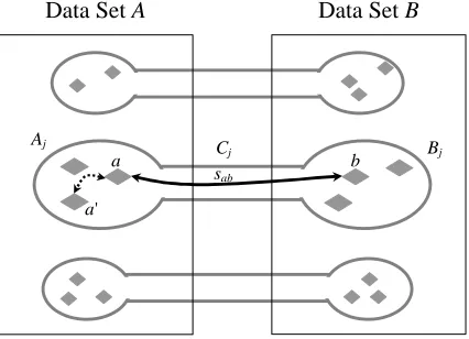
Coupled clustering divides two given data sets denoted by A and B into disjoint subsets A1, …, Ak and B1, …, Bk. Each of these subsets is coupled with the corresponding subset of the other data set, that is Aj is coupled with Bj for j = 1…k. Every pair of coupled subsets forms a unified coupled cluster, Cj = AjΥBj, containing elements of both data sets (see Figure 3). We approach the coupled clustering problem through a pairwise-similarity-based setting, incorporating the elements of both A and B. Our treatment is independent of the method through which similarity values are compiled: feature-based calculations such as those described in Subsection 2.2, subjective assessments, or any other method.

The notable feature distinguishing our method from standard pairwise clustering, is the set of similarity values, S, that are considered. A standard pairwise clustering procedure potentially considers all available similarity values referring to any pair of elements within the single clustered data set, with the exception of the typically excluded self-similarities. In the coupled clustering setting, there are two different types of available similarity values. Values of one type denote similarities between elements within the same data set (within-data-set similarities; short arrow in Figure

Data Set A

Aj

a b

sab

Data Set B

Bj

a'

Cj

(10)

3). Values of the second type denote similarities of element pairs consisting of one element from each data set (between-data-set similarities; long arrow in Figure 3). As an initial strategy, to be complied with throughout this paper, we choose to ignore similarities of the first type altogether and to concentrate solely on between-data-set similarities: S = {sab}, where a∈A and b∈B. Consequently, the assignment of a given data element into a coupled cluster is directly influenced by the most similar elements of the other data set, regardless of its similarity to members of its own data set.

The policy of excluding within-data-set similarities captures, according to our conception, the unique context posed by aligning two data sets representing distinct domains with respect to one another. Correspondences, underlying presumed parallel or analogous structure of the compared systems, that are special to the current comparison are thus likely to be identified, abstracted from the distinctive information characterizing each system individually. Whether and how to incorporate the available information regarding within-data-set similarities, while maintaining the contextual orientation of our method is left to a follow up research.

3.3. Three Alternative Cost Functions

Given the setting described above, in order to identify configurations that accomplish the coupled clustering task, our next step is defining a cost function. In formulating it, we closely follow the standard pairwise-clustering framework presented by Puzicha, Hofmann and Buhmann, (2000, see Subsection 2.1 above). Given a collection of similarity values S pertaining to the members of two data sets, A and B, we formulate an additive cost function, H(S,M), which assigns a cost value to any coupled-clustering configuration M. Equipped with such a cost function and a search strategy (see Subsection 3.4 below), our procedure would be able to output a coupled clustering configuration specifying assignments of the elements into a pre-determined number, k, of coupled clusters. We concentrate on Puzicha et al.'s H0 cost function (Subsection 2.1, Equation 6), which is limited to similarity values within each cluster and weights each cluster's contribution proportionally to its size. Below we present and analyze three alternative cost-functions derived from H0.

As in clustering in general, the coupled clustering cost function should assign similar elements into the same cluster and dissimilar elements into distinct clusters (as articulated by the monotonicity axiom in Subsection 2.1). A coupled-clustering cost function is thus expected to assign low cost to configurations in which the similarity values, sab, of elements a and b of coupled subsets, Aj and Bj, are high on average. (The dual requirement to assign low cost whenever similarity values of elements a and b of non-coupled subsets Aj and Bj', j≠j', are low, is implicitly fulfilled). In addition, we seek to avoid influence of transient or minute components—those that could have been evolved from casual noise or during the optimization process—and maintain the influence of stable larger components. Consequently, the contribution of large coupled clusters to the cost is greater than the contribution of small ones with the same average similarity. This direction is realized in H0 through weighting each cluster's contribution by its size.

In the coupled-clustering case, one apparent option is to straightforwardly apply the original H0 cost function to our restricted collection of similarity values. The average similarity of each cluster is then calculated as

) 1 (

' ,

− ×

=

∑

∈ ∈

j j

B b A a ab j

n n

s

(11)

where nj is the total size of the coupled cluster Cj. (This is equivalent to setting to 0 all within-data-set similarities in Equation 5). As in H0, the average similarity of each cluster is multiplied by the coupled-cluster size. Thus, the following cost function, H1, is obtained:

H1=−

∑

jnj ×Avg'j . (10)

Alternatively, since the calculations are limited to a restricted collection of similarities, we can incorporate the actual size of the similarity collection in use while averaging. The actual number of considered similarities in the restricted collection is, for each j, the product B

j A j n

n × _{of the sizes of the two subsets}_A_j_and_B_j_composing_C_j_. The obtained averaging formula might seem more natural for the purpose of coupled clustering: B j A j B b A a ab j n n s

Avg j j

× =

∑

∈ ,∈

'

' ,

Correspondingly, a second cost variant, H2, is given:

H2=−

∑

jnj ×Avg"j. (11)

However, the weighting scheme used within H1and H2 treats each coupled cluster as a unified object. There might be some significance to the proportion of the subset sizes that are coupled within each cluster. Hence, we suggest yet another alternative: to weight the average similarity each cluster contributes to the cost by the geometrical mean of the corresponding coupled subset sizes: B

j A j n

n × . This yields our last cost function:

H3=−

∑

j

B j A j n

n × ×Avg"j . (12)

The weighting factor of H3 results in penalizing large gaps between the two sizes, A j

n

and B j

n _{, and in preferring balanced configurations, whose coupled-cluster inner} proportions maintain the global proportion of the clustered data sets ( B

j A j n

n ≅ A

n

/

B

n

for each j).

Puzicha, Hofmann and Buhmann, (2000) based their characterization of pairwise- clustering cost-functions on some properties and axioms (see Subsection 2.1 above). We have followed their conclusions in adapting, in three different variants, one function, H0, that realizes the most favorable properties. It is worthwhile to see if and how these properties are preserved through the adaptation for the coupled clustering setting. All three cost functions obtained, H1, H2 and H3, are additive (Equation 1) by construction. They also straightforwardly satisfy the scale invariance property (Equation 2). As for shift-invariance (Equation 3), except by H2, this property is not fulfilled. However, the effect of a constant added to all between-data-set similarity values is bounded for H1and H3, as well4. Finally, robustness (Equation 4) is satisfied by H1and H3 (but not by H2, see Appendix A).

Using the coupled sizes' geometrical mean as a weighting factor, H3 tends to escape configurations whose clusters match minute subsets with large ones, which are

4

To check shift-invariance, one can use the derivative of, say, H3 with respect to ∆, which is the increment for all between-data-set similarity values. This is a linear function so the resulting derivative is D = j B

j A j n n ×

1

Consequently, normalizing H3_by_1/_D_{would result in perfect shift invariance. However, this function, in its}

(12)

occasionally the consequence of noise in the input data or of fluctuations in the search process. It turns that this property provides H3 with a notable advantage over H1and H2, as our experiments indeed show (see Sections 4, 5.2 and 6).

3.4. Optimization Method

In order to find the clustering configuration of minimal cost, we have implemented a stochastic search procedure, namely the Gibbs sampler algorithm (Geman and Geman, 1984). Starting with random assignments into clusters, this algorithm iterates repeatedly through all data elements and probabilistically reassigns each one of them in its turn, according to a probability governed by the expected cost change. Suppose that in a given assignment configuration, M, the cost difference ∆_j|a,M is obtained by reassigning a given element, a, into the j-th cluster (∆_j|a,M= 0 in case a is already assigned to the j-th cluster). The target cluster, into which the reassignment is actually performed, is selected among all candidates with probability

p(j) ≡ p(j|a,M) π

} exp{

1

, |aM j ∆ −

+ β .

Consequently, the chances of an assignment to take place are higher as the resulting reduction in cost is larger. In distinction from the similar Metropolis algorithm (Metropolis et al., 1953), assignments that result in increased cost are possible, though with relatively low probability. The β parameter, controlling the randomness level of reassignments, functions as an inverse “computational temperature”. Starting at high temperature followed by progressive cooling schedule, that is initializing β to a small positive value and gradually increasing it (e.g., repeatedly multiply β by a constant that is slightly greater than one), turns most profitable assignments increasingly probable. As the clustering process proceeds, gradual cooling systematically reduces the probability that the algorithm would be trapped in a local minimum (though global minimum is fully guaranteed only under an impracticably slow cooling schedule). In our experiments, we have typically initialized β to the mean of the data set sizes divided by the cost of the initial configuration and multiplied β by a factor of 1.001, following every iteration in which improvement in cost has been achieved. The algorithm stops after several repeated iterations through all data elements, in which no cost change has been recorded (50 iterations in our experiments).

4. Experiments with Synthetic Data

A set of experiments on synthetic data has been conducted for comparing the performance of our algorithm, making use of the three cost functions introduced in Subsection 3.3 above. These experiments have measured, under changing noise levels, how well each of the functions reconstructs a configuration of pre-determined clusters of various inner proportions.

(13)

In precise terms, the similarity value sab, of any a∈A and b∈B (A and B are the clustered data sets), has been set to

sab = (1−x)δj(a)j(b) + xrab ,

where δj(a)j(b)—the basic similarity level—is 1 if a∈A and b∈B are, by construction, in the same (j-th) coupled cluster or otherwise 0 and rab—the random component—is sampled uniformly between 0 and 1, differently for each a and b in each experiment. The randomness proportion parameter x (i.e. level of added noise), also between 0 to

1, is fixed throughout each experiment, to keep the noise level of each experiment unaltered.

In order to study the effect of the coupled-cluster inner proportion, we have run four sets of experiments. Given data sets A and B consisting of 32 elements each, four types of synthetic coupled-clustering configurations have been constructed, in which the sizes A

j

n _and B j

n _{of the coupled subset pairs}_A_j⊂_A_and_B_j⊂_B_{, together forming the}

j-thcoupled-cluster, have been set as follows: (i) A j

n = B

j

n =_{8, for}_j_{= 1…4; (ii)} A j

n =_10,

B j

n =_{6 for}_j_{= 1,2 and}nAj = 6,

B j

n =_{10 for}_j_{= 3,4; (iii)}nAj = 12,

B j

n =_{4 for}_j_{= 1,2 and}nAj = 4, B

j

n =_{12 for}_j_{= 3,4; (iv)} A j

n =_14, B j

n =_{2 for}_j_{= 1,2 and} A j

n =_2, B j

n =_{14 for}_j_{= 3,4.} These four configuration types, respectively labeled ‘8-8’, ‘10-6’, ‘12-4’ and ‘14-2’, have been used in the four experiment sets.

(14)

It is convenient to visualize a collection of similarity values as a gray-level matrix, where rows and columns correspond to individual elements of the two clustered data sets and each pixel represents the similarity level of the corresponding elements. The diagrams on the left-hand side in Figure 4 show two collections of similarity values generated with two different noise levels. White pixels represent the maximal similarity level in use, 1; black pixels represent the minimal similarity level, 0; the intermediate gray levels represent similarities in between. The middle and right-hand-side columns of Figure 4 display clustering configurations as reconstructed by our algorithm using the additive H2 and multiplicative H3 cost functions respectively, given the input similarity values displayed on the left-hand side. Examples from the 10-6 experiment set, with two levels of noise, are displayed. Bright pixels indicate that the corresponding elements are in the same reconstructed cluster. It demonstrates that, for the 10-6 inner proportion, the multiplicative variant H3 tends to tolerate noise better than the additive variant H2 and that this advantage grows when the noise level intensifies (bottom of Figure 4).

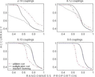
The performance over all experiments in each set has bean measured through accuracy, which is the proportion of data elements assigned into the appropriate coupled cluster. Since in cases of poor reconstruction it is not obvious how each reconstructed cluster associates with an original one, the best result obtained by permuting the reconstructed clusters over original clusters has been considered. Figure 5 displays average accuracy for the changing noise levels, separately for each experiment set. The multiplicative cost function H3, is biased toward balanced coupled clusters, i.e. clusters in which the inner proportion is close to the global proportion of the data sets (which is perfectly balanced, 32-32, in our case). Our

(15)

experiments indeed verify that H3 reconstruct better than the other functions, particularly in cases of almost balanced inner proportions.

Figure 5 shows that the accuracy obtained using the restricted standard-clustering function H1 is consistently worse than the accuracy of H3. In addition, for all internal proportions, there is some range, on the left-hand side of each curve, in which H3 performs better than the additive function H2. The range where H3 is superior to H2 is almost unnoticeable for the sharply imbalanced internal proportion (2-14) but becomes prominent as the internal proportion approaches balance. Consequently, it makes sense to use the additive function H2 only if both: (i) there is a good reason to assume that the data contains mostly imbalanced coupled clusters and (ii) there is a reason to assume high level of noise. Real world data might be noisy, but given no explicit indication that the emerging configurations are inherently imbalanced, the multiplicative function H3 is preferable. Consequently, we have used H3 in our experiments with textual data, described in the following sections.

5. Coupled Clustering for Textual Data

In this section, we demonstrate capabilities of the coupled clustering algorithm with respect to real-world textual data, namely unstructured sets of keywords (corresponding to data sets A, B of Subsection 3.3). The keywords have been extracted from given corpora focused on distinct domains. Our experiments have been motivated by the target of identifying concepts that play similar or analogous roles in the examined domains. These experiments examine how well coupled clusters produced by our method reflect such conceptual equivalencies. Our results demonstrate meaningful and interesting semantic correspondences of themes, entities and categories revealed through coupled clustering.

Our setting assumes that the data sets are given or can be extracted automatically. We have used the TextAnalyst 2.0 software by MicroSystems Ltd.5 to generate data sets for our experiments. This software can identify key-phrases in the given corpora. We have excluded the items that have appeared in fewer than three documents. Thus, relatively rare terms and phrases that the software has inappropriately segmented have been filtered out.

After extracting the data sets, between-data-set similarities, if not given in advance, should be calculated. In general terms, every extracted keyword is represented by a co-occurrence vector, whose entries essentially correspond to all co-occurring words (concrete examples follow in the subsections bellow), less a limited list of function words. Then, between-data-set similarity values are calculated using methods, such as those described in Subsection 2.2, to adapt the data for the coupled-clustering algorithmic setting introduced in Subsection 3.2. We differentiate between two optional sources that can provide the co-occurrence data for the similarity calculations. One option is to base the calculations on co-occurrences within the same corpora from which the keyword sets have been extracted. Thus, the calculated similarity values naturally reflect the context in which the comparison is being made. However, sometimes the compared corpora might be of small size and there is a need to rely on a more informative statistical source. An alternative option is to utilize the co-occurrences within an additional independent corpus for the required similarity calculations. In order to produce reliable and accurate similarity values, such independent corpus can be chosen to be significantly larger than the compared ones,

5

(16)

but it is important that it addresses well the topics that are being compared, so the context reflected by the similarities is still relevant.

The following subsections provide results that have been obtained using the two approaches described above. In Subsection 5.1, the keyword sets come from news articles referring to two conflicts of different character that are nowadays in the focus of public attention. In this case, we make use of pre-given word similarity values. In Subsection 5.2, we turn to larger corpora focused on various religions. There, keywords and co-occurrence counts underlying similarity calculations are extracted from the same corpora.

5.1. Coupled Clustering of Conflict Keywords Using Pre-given Similarities The conflict corpora are composed of about 30 news articles each (200–500 word tokens in every article), regarding the two conflicts mentioned in Section 1—the Middle East conflict and the dispute over music copyright—downloaded in October 2000.

We have obtained the similarities from a large body of word similarity values that have been calculated by Dekang Lin, independently of our project (Lin, 1998). Lin has applied the simL similarity measure (Subsection 2.2, Equation 9) to word

co-occurrence statistics within syntactic relations, extracted from a very large news-article corpus.6 We assume that this corpus includes sufficient representation of the conflict keyword sets in relevant contexts. That is: even if the articles in the corpus do not explicitly discuss the concrete conflicts, it is likely that they address similar issues, which are rather typical as news topics. In particular, occurrences of the clustered keywords within this corpus are assumed to denote meanings resembling their sense within our small article collection that might not provide sufficiently rich statistics for extracting this information due to its limited size.

As Table 1 shows, the coupled-clusters that have been obtained by our algorithm fall, according to our classification, within three main categories: “Parties and Administration”, “Issues and Resources in Dispute” and “Activities and Procedure”. To improve readability, we have also added an individual title to each cluster.

The keywords labeled “poorly-clustered”,at the bottom of Table 1, are assigned to a cluster with average similarity considerably lower than the other clusters, or for which no relevant between-data-set similarities are found in Lin's similarity database. Consequently, these keywords could be straightforwardly filtered out. However, poorly clustered elements persistently occur in most of our experiments and we include them here for the sake of conveying the whole picture.

Making use of pre-given similarity data is, on the one hand, trivially advantageous. Apart from saving programming and computing resources, such similarity data typically relies on rich statistics and its quality is independently verified. Moreover: in principle, pre-given similarity data could be utilized for further experiments in clustering additional data sets that are adequately represented in the similarity database. However, there are several disadvantages in taking this route. First, reliable relevant similarity data is not always available. In addition, the context of comparing two particular domains might not be fully articulated within generic similarity data that has been extracted in a much broader context. For example, the interesting case where the same keyword appears in both clustered sets, but it is used for different meanings, could not be traced. A keyword used differently in distinct corpora would co-occur with different features in each corpus . In contrast, when similarities are

6

(17)

Table 1:Coupled clustering of conflict related keywords. Every row in the table contains the keywords of one coupled cluster. Cluster titles and titles of the three groups of clusters were added by the authors.

Middle-East Music Copyright

Parties and Administration

Establishments _{city state} _{company court industry university}

Negotiation _{delegation minister} _{committee panel}

Individuals _{partner refugee soldier terrorist} _student

Professionals _{diplomat leader} _{artist judge lawyer}

Issues and Resources in Dispute

Locations _{home house street} _{block site}

Protection _{housing security} _{copyright service}

Activity and Procedure

Resolution _{defeat election mandate meeting} _decision

Activities1 _{assistance settlement} _{innovation program swap}

Activities2 _{disarm extradite extradition face} _use

Confrontation _attack _{digital infringement label shut violation}

Communication _{declare meet} _{listen violate}

Poorly-clustered keywords

low similarity

values interview peace weapon existing found infringe listening medium _{music song stream worldwide}

No similarity

values armed diplomatic

computed from a unified corpus, self-similarity is generally equal to the highest possible value (1 in Lin's measure), which is typically much higher than other similarity values. In such case, the two distinct instances of a keyword presenting in both clustered sets would always fall within the same coupled-cluster

5.2. Clustering of Religion Keywords with Dedicated Similarity Calculations

(18)

informative. In summary, while the use of pre-given similarity data takes advantage of richer statistics over a unified set of features, the other alternative analyzes keywords in their more appropriate and accurate sense. It makes sense to use this approach whenever a sufficient amount of shared features and rich statistics are present, as exemplified below.

We have applied our method to corpora that discuss distinct religions in order to compare these religions to one another and to identify corresponding concepts within them. The religion data consists of five corpora, each of which focuses on one of the following religions: Buddhism, Christianity, Hinduism, Islam and Judaism. All documents, namely encyclopedic entries, electronic periodicals and additional introductory web pages, have been downloaded from the Internet. Each corpus contains 1–1.5 million word tokens (5–10 Megabyte).

Keywords that have been provided by comparative religion experts are included in the data sets, in addition to the keywords extracted by the TextAnalyst 2.0 software (the expert data has been primarily used for quantitative evaluation, see Section 6). The total size of each of the final keyword sets is 150–200, of which 15–20% were not extracted by TextAnalyst, but solely by the experts.

Each keyword has been represented by its co-occurrence vector as extracted from its own corpus. In counting co-occurrences, we have used two-sided sliding window of ±5 words, truncated by sentence ends (similarly to Smadja, 1993). On one hand, this window size captures most syntactic relations (Martin, Al and van Sterkenburg, 1983). On the other hand, this scope is wide enough to score terms that refer to the same topic in general—and not only literally interchangeable terms—as similar (Gorodetsky, 2001), which is in accordance with our aim of identifying corresponding topics. We have applied to the obtained vectorial representations the simDMM similarity

measure, which incorporates detailed information on the data (Dagan, Marcus and Markovitch 1995; Subsection 2.2, Equation 8: simDMM incorporates maximal and

minimal information values for each common feature individually; simL is less

detailed in that it separately sums maximal values versus minimal values). After calculating between-data-set similarities, we ran the coupled clustering algorithm on each dataset pair.

In Table 2, we present the full coupled-clustering results for Buddhism versus Christianity. The keyword sets are partitioned into 16 coupled clusters, ordered by their average similarity in descending order. The poorly clustered elements, i.e. those contained in the 16th cluster with the lowest average similarity, are not shown. We attach intuitive titles to each cluster for readability and orientation. The obtained clusters (and also additional results that are not shown concerning other religion pairs) appear to reflect consistently several themes:

• Holy books, writing, teaching, and studying.

• Individual figures and their characteristics.

• Names of places and institutions.

• Ethics, emphasizing sins and their consequences.

• Traditions and schools.

• Festivals.

(19)

Table 2: Coupled clustering of Buddhism and Christianity keywords. Cluster labels were added by the authors. The 16th cluster of lowest average similarity is not shown.

Buddhism Christianity

1. Schools and Traditions

doctrine, establish, ethic, exist, Hindu, India, Mahayana, scholar, school, society, study, Zen

catholic, history, Protestant, religion, tradition

2. Scripture and Theology

book, question, religion, text, tradition, west

apostle, bible, book, doctrine, Greek, Jew, john, question, scripture, theology, translate, write

3. Sin / Suffering cause, death, Dukkha, pain death, flesh, Satan, sin, soul, suffer

4. Founder Characteristics

being, Buddha, experience, meditation, monk, sense, teaching

believe, child, church, faith, find, god, Jesus Christ, Paul, pray, word

5. Mental States animal, attain, awaken, awareness, Bodhisattva, consciousness, disciple, enlightenment, existence, karma, mindfulness, moral, nirvana, realm, rebirth, speech, Tantra, teach, word

baptism, experience, moral, problem, relationship, teaching

6. Approach to the Religious Message

find, hear, learn, problem baptize, born, disciple, friend, gentile, hear, hell, judge, judgment, king, lost, love of god, Mary, preach, prophet, sacrifice, savior, sinner, story, teach

7. Locations / Figures / Ritual

country, king, monastery, Sangha, temple

angel, authority, city, Israel, Jerusalem, priest, saint, service, Sunday, worship

8. Central Symbols and Values

Dharma, god, peace, wisdom bless, cross, earth, gift, heaven, holy ghost, kingdom, peace, resurrection, revelation, righteousness, salvation

9. Studying ascetic, Bhikkhu, discipline, friend, Gautama, guide, philosopher, student, teacher

learn, minister, study, teacher

10. Commands, Sin and Punishment

anger, kill, law adultery, command, commandment,

forgiveness, law, punish, repentance

11.

Philosophical Concepts

emptiness, foundation, four noble truths, phenomena, philosophy, soul, theory

argue, argument, foundation, humanity, incarnation, trinity

12. Traditions and their Origins

Asia, china, founded, Japan, north, nun, pilgrim, Theravada, Tibet

Baptist, bishop, establish, member, ministry, orthodox

13. Holy Books discourse, history, Lama, mandala, Pali canon, Sanskrit, scripture, story, sutra, translate, Tripitaka, Vinaya, write

author, gospels, Hebrew, New Testament, Old Testament, passage, writing

14. Customs and Rituals

Amida, gift, mantra, purity, sacrifice, spirit, worship

atonement, confession, Eucharist, good works, pilgrim, reward, sacrament

15. Figures, Festivals, Holy Places

Dalai Lama, Korea, Sri Lanka, writing Christmas, Easter, Good Friday, Isaiah, Luke, mass, Matthew, monk, Pentecost, Pope, Rome, university, Vatican

Furthermore, the displayed keyword coupled clusters reveal differences and variations between the compared religions that seem to us of particular interest:

(20)

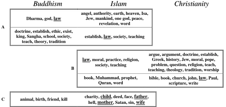
data sets; see Figure 6A). The particular assignments are related with different senses. In Christianity, the sense is of written law and holy books, such as the laws of religion. In Islam, it is related to philosophical laws that require learning and understanding. In the Buddhism–Islam comparison, the senses differ even more sharply (Figure 6B): in Buddhism the term law stands for the message of God or “law of nature”. In Islam, it is related with social law, and with education, as well.

• Family relations. Family relations seem to be important in Islam. In the obtained Buddhism–Islam clustering configuration, the related cluster is associated with few additional Islamic terms, concerning inter-personal relationships and ethics. The Buddhist terminology seem to be less developed with respect to these aspects (Figure 6C).

• Religion founder. The key-figures of each religion are consistently assigned to a cluster associating them with prominent themes of the particular religion. Buddha, for instance, is characterized by ‘being’, ‘meditation’ and ‘teaching’, Jesus—by ‘believing’ and ‘prayer’ and Muhammad—by ‘Quran’ and ‘worship’. We provide further qualitative evaluation of results concerning comparison of religions in Section 6 below.

6. Evaluation

In order to evaluate textual coupled clustering results, such as those presented in Section 5 above, we have asked human subjects whose academic field of expertise is the comparative study of religions to manually perform a coupled clustering task. We have asked the experts to point, without any restriction, the most prominent equivalent aspects common to given pairs of religions. (To convey a broad notion of equivalency, we have included the following phrase in the instructions: “… features and aspects that are similar, or resembling, or parallel, or equivalent, or analogous in the two religions under examination…”). Then, every expert has been requested to specify some freely chosen representative terms that characteristically address the

B

u

d

h

i

s

m

I

s

l

a

m

C

h

r

i

s

t

i

a

n

i

t

y

Dharma, god, law

angel, authority, earth, heaven, Isa, Jew, mankind, one god, peace,

revelation, word A

doctrine, establish, ethic, exist, king, Sangha, school, society,

teach, theory, tradition

establish, law, society, teaching

law, moral, practice, religion, society, teaching

argue, argument, doctrine, establish, Greek, history, Jew, moral, pope, problem, question, religion, teach, teaching, theology, tradition, worship B

book, Muhammad, prophet, Quran, word

bible, book, church, john, law, Paul, scripture, write

C animal, birth, friend, kill charity, child, deed, face, father, hell, mother, Satan, sin, wife

(21)

identified similar aspects within the content world of each of the compared religions. For the purposes of the evaluation, the union of each resulting pair of corresponding sets of terms, separately addressing one aspect of similarity in two distinct religions, is defined to be a unified coupled-cluster. Example of aspects shared by Buddhism and Islam, as suggested by one of the experts, together with the associated terms specified by this expert can be seen in the first lines of Table 3.

Coupled clustering is a newly defined computational framework and no well-established means for evaluating its outcome are available. In the absence of objective criteria, we have found it appropriate to evaluate our procedure by measuring how well it approximates the keyword clustering-configurations produced by the human experts. We have let the participants choose the number of clusters for each religion pair, as well as the specific terms included in every cluster. Thus, our evaluation is free from bias that could have emerged due to restricting the experts to certain aspects of similarity or to a given list of keywords extracted in one method or another. For evaluation purposes, the two keyword sets, to be clustered by the computerized procedure in each case, have included the terms presented by the experts, excluding terms that are absent or rarely found in our corpora. These rare terms have been excluded also from the expert clusters, to allow unified grounds for comparison. The required similarity values have been calculated based on co-occurrence data extracted from the religion corpora (as in Subsection 5.2).

The measure of overlap between expert and automated clustering configurations is based on counting pairs of keywords consisting of one element from each of the clustered keyword sets. Specifically, we have used the Jaccard coefficient, which is in common use for evaluating information retrieval and clustering results (e.g., Ben-Dor, Shamir, & Yakhini, 1999). In the coupled clustering case, given clustering configurations by both expert and our computerized procedure, the Jaccard coefficient is defined as

01 10 11

11

n n n

n

+

+ ,

where

n11 – the number of pairs of keywords, one of each data set, that have been assigned

by both the expert and our program into the same cluster;

n01 – the number of keyword pairs that have been assigned into the same cluster by

the expert but not by our program;

n10 – the number of keyword pairs that have been assigned into the same cluster by

our program but not by the expert.

(22)

The Jaccard coefficient is used to check the overlap of the clustering configurations obtained using the multiplicative cost function H3 (Subsection 3.3, Equation 12; H3 has been used also in Section 5) with expert configurations. This overlap level is compared to a simple benchmark: the expected coefficient obtained from the overlap between the experts configurations and configurations consisting of random assignments of elements into clusters. In addition, we compare the overlap of the expert configurations with results obtained using the additive cost function H2 (Equation 11) to experts vs. multiplicative cost function overlap and experts vs. random assignment overlap. The overlap between different experts has also been recorded in all cases where different experts have provided configurations referring to the same pair of religions.

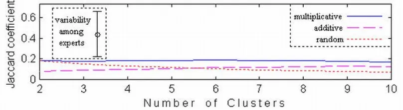
Figure 7 displays a sample of the Jaccard coefficient values measuring the overlap of six of the 17 configurations contributed by religion experts with the corresponding configurations due to the multiplicative and additive functions, as well as random assignments. The selection of six configurations has been chosen to represent, in a conveniently displayable manner, the various trends that were found with regard to the overlap of our automated configurations of 2 to 10 coupled clusters with the expert data. The displayed Jaccard coefficient values demonstrate that there is no

(23)

priory known optimal number of clusters that would yield the best results. The optimum is obtained for various cluster numbers, which are not tightly related to the number of expert clusters (the cause of this empirical mismatch requires yet a further examination). However, over the whole displayed selection, we see that the multiplicative cost function in general shows superior performance compared to both additive function and random assignments. In some cases, there is a local maximum on the multiplicative function curve, additional to the global maximum, indicating that there is more than one meaningful resolution fitting the data.

In Figure 8, the Jaccard coefficient is averaged, separately for each number of our output clusters, over all comparisons to expert configurations (each with its own fixed number of expert clusters). Thus, we ignore optimal numbers of clusters obtained for each particular comparison (demonstrated for six cases by Figure 7). The overlap of expert configurations with random assignments decreases with the number of clusters, since randomness trivially dominates, as more clusters are added. In distinction, overlap with the additive cost configurations increases with the number of clusters. The additive function performs poorly in cases of fewer and larger clusters, because of its bias towards imbalanced couplings. The multiplicative function is shown to maintain its superiority consistently over the whole range. Figure 8 displays also some indication of variability among experts. Note that there have been only eight cases of identical religion pairs compared by distinct experts. In each of these cases, the overlap is measured on keyword sets that are considerably smaller than the original expert sets, since the distinct expert configurations do not share large proportion of common terms. It can be seen that one standard deviation below the average overlap among the experts is close to the average overlap level obtained by the multiplicative function.

For overall quantitative assessment of the results, we average over the Jaccard coefficient values obtained with 2 to 10 clusters, separately for each expert configuration and each assignment method. Thus, three corresponding sets are obtained, each related with another assignment method, containing 17 representative values each, which are assumed independent within each sample. We hypothesize that the difference between the corresponding values in these three sets is not coincidental. The difference between multiplicative cost and random average results, taken individually for each expert clustering configuration, is indeed statistically significant (x = 0.067, t(16) = 5.53, p < 0.00005). Superiority of the multiplicative cost on the additive cost is even more significant (x = 0.070, t(16)= 13.98, p < 10−8), because these cost functions involve the same similarity data, they

Figure 8: Average trends of three reconstruction methods—multiplicative H3, additive H2

(24)

Table 3: A coupled clustering configuration regarding the mapping between Buddhism and Islam contributed by one of the experts (A) followed by the output of computerized procedures: coupled clustering using the multiplicative, H3 (B) and additive, H2 (C) cost functions and standard clustering, H0 (D) – applied to the same keywords.

Buddhism Islam

A. Expert coupled clustering

Scripture _{koan, mantra, mandala, pali canon, sutra hadith, muhammad, quran, sharia, sunna}

Beliefs and

ideas buddha nature, dharma, dukkha, _{emptiness, four noble truths, nirvana,}

reincarnation

allah, five pillars, heaven, hell, one god

Ritual, prayer

and festivals gift, meditation, sacrifice, statue, stupa charity, fasting, friday, id al fitr, kaaba, _{mecca, pilgrim, pray, ramadan}

Mysticism _{samadhi, tantra} _sufi

B. Multiplicative cost function

dharma dukkha, meditation allah, muhammad, pray, quran