Galley
Pro
of
Iranian Journal of Numerical Analysis and Optimization Vol. 7, No. 2, (2017), pp 115–135
DOI:10.22067/ijnao.v7i2.62042
Using a LDG method for solving an
inverse source problem of the
time-fractional diffusion equation
S. Yeganeh, R. Mokhtari∗ and S. Fouladi
Abstract
In this paper, we apply a local discontinuous Galerkin (LDG) method to solve some fractional inverse problems. In fact, we determine a time-dependent source term in an inverse problem of the time-fractional diffusion equation. The method is based on a finite difference scheme in time and a LDG method in space. A numerical stability theorem as well as an error estimate is provided. Finally, some numerical examples are tested to confirm theoretical results and to illustrate effectiveness of the method. It must be pointed out that proposed method generates stable and accurate numerical approximations without using any regularization methods which are neces-sary for other numerical methods for solving such ill-posed inverse problems.
Keywords: Local discontinuous Galerkin method; Inverse source problem; Time-fractional diffusion equation.
1 Introduction
Recently, studying problems involving fractional order partial differential equations (PDEs) has attracted a lot of interests of scientists and engi-neers, see e.g. [1, 5–12, 15, 18–20, 22, 24–30, 33–35]. One of the fractional ∗Corresponding author
Received 22 January 2017; revised 29 March 2017; accepted 23 April 2017 S. Yeganeh
Department of Mathematical Sciences, Isfahan University of Technology, Isfahan 84156-83111, Iran. e-mail: [email protected]
R. Mokhtari
Department of Mathematical Sciences, Isfahan University of Technology, Isfahan 84156-83111, Iran. e-mail: [email protected]
S. Fouladi
Department of Mathematical Sciences, Isfahan University of Technology, Isfahan 84156-83111, Iran.
Galley
Pro
of
PDEs which has been very popular is the fractional diffusion equation (FDE), see e.g. [1, 6–12, 15, 18–20, 22, 24–30, 33–35]. Nowadays instead of the classi-cal diffusion equations, FDEs have attracted wide attentions since a FDE is a generalization of a diffusion equation which can be used to describe an anomalous diffusion phenomenon such as super-diffusion or sub-diffusion. By replacing the standard time derivative with a time fractional derivative in a diffusion equation, a time-fractional diffusion equation is obtained. FDEs can be applied in modelling of some problems in porous flows, rheology and mechanical systems, models of a variety of biological processes, control and robotics, transport in fusion plasmas, and many other areas of applications. Analytical or numerical studying of the direct problems corresponding to the time-fractional diffusion equations have been carried out extensively in the recent years, see e.g. [6, 7, 9, 11, 12, 15, 30] as well as references cited therein [27, 28] for some subjects related to the obtaining some uniqueness and existence results, establishing maximum principle, finding analytical so-lutions, applying some numerical methods such as finite element methods or finite difference methods.
If in an initial or initial-boundary value problem some parts of data such as boundary data, or initial data, or source term or even some coefficients of the main equation may not be given, we have encountered an inverse problem. Inverse problems are appeared in many practical situations, and for solving them we need to some additional measured data, see e.g. [1,8,10,16–25,27–29, 32–35] and references cited therein. In some inverse problems, we need to find space-dependent source term [27, 32] or time-dependent source term [28] or even space- and time-dependent source term [23]. In this paper, we focus our attention on finding the time-dependent source term in a fractional inverse problem which is one of the interesting and novel inverse problems. One of the pioneering scientists in this subject is Murio [18–20]. In the following we mention some of works which have been published after that. An inverse problem for determining the order of fractional derivative and the diffusion coefficient in a FDE has been considered in [1] where a uniqueness result has been also obtained. A backward problem for the time-fractional diffusion equation has been solved by a quasi-reversibility regularization method in [13]. In [34, 35] some Cauchy problems based on the time-fractional diffusion equation have been investigated on a bounded domain and on a strip domain, respectively. Qian [22] has investigated a modified kernel method for solving an inverse fractional diffusion equation. An inverse source problem for a FDE has been solved in [33]. Rundell et al. [10] have been investigated some nonlinear fractional inverse problems. Recently, some interesting works have been carried out by Wei et al., see e.g. [27–29]. In [10] known theoretical results and computational techniques for FDEs have been provided.
Galley
Pro
of
Using a LDG method for solving an inverse source problem ... 117
Dα
tu=uxx+f(x)p(t),0< x <1,0< t < T,
u(0, t) =k0(t), 0⩽t⩽T, u(1, t) =k1(t), 0⩽t⩽T, u(x,0) =ϕ(x), 0⩽x⩽1,
(1)
whereDαt is the Caputo fractional derivative of orderα, i.e.,
Dtαu= 1 Γ(1−α)
∫ t
0
∂u(x, s)
∂s
ds
(t−s)α, 0< α <1, (2)
in which Γ is the Gamma function. Forα= 1, we haveDα
tu=ut. We assume
thatk0,k1 andϕare given functions. Problem (1) will be a direct (forward)
problem wheneverf andpare known functions. Based on the availability of
f orp, there are some inverse problems. Ifpis known and f is unknown we need to an extra condition such as
u(x, T) =g(x), 0≤x≤1.
We have investigated numerical solution of this inverse problem in [32]. In another inverse problem, f is known but p is unknown and an over-determination condition such as
u(x∗, t) =g(t), 0≤t≤T, (3)
will be needed wherex∗∈(0,1) is an interior measurement location. It must be pointed out that although these two inverse problems are very similar they are completely different. The inverse source problem which we consider here is to determine (p, u) based on problem (1) and condition (3). Using the main equation in (1) and Eq. (3), we have
p(t) = 1
f(x∗)
(
Dαtg(t)−∂
2u(x∗, t) ∂x2
)
. (4)
We need (4) just for theoretical purposes.
Galley
Pro
of
results, see e.g. [32] where a space-dependent source term is determined in a time-fractional diffusion equation by using a local discontinuous Galerkin method. Of course, some DG methods have been applied successfully for the forward fractional diffusion equation. For example, Hesthaven et al. [6, 30] have been solved some space-fractional diffusion equations using a local dis-continuous Galerkin method in a semi-discrete regime and Yang Liu et al. [14] have developed a LDG methos combined with WSGD approximation for a time fractional subdiffusion equation.
In the present paper, we aim to extend application of the discontinuous Galerkin method to some inverse source problems and for this purpose, we present a fully-discrete local discontinuous Galerkin method for solving the inverse source problem of the time-fractional diffusion equation. In the pro-posed fully-discrete method, we apply a LDG method for the space variable and the time-fractional derivative is discretized by using a backward differ-ence scheme. The rest of the paper is organized as follows. In Section 2, some preliminaries are prepared. Construction of the proposed method for the inverse source problem (1)-(3) as well as stability and convergence the-orems are dealt with in Section 3. Section 4 is devoted to some numerical experiments to illustrate the accuracy and capability of the method. Finally, the paper is concluded with a brief conclusion.
2 Preliminaries
In this section, some notations are defined and some auxiliary results are prepared. At first, we decompose interval [0,1] to some cells (subintervals) as follows
0 =x1 2 < x
3
2 <· · ·< xN+ 1 2 = 1, and set Ij = [xj−1
2, xj+ 1
2], with the cell lengths ∆xj = xj+ 1 2 −xj−
1 2, for
j = 1, . . . , N and h = max1≤j≤N∆xj. We denote by u+j+1 2
and u−j+1 2
the values ofuatxj+1
2,from the right cellIj+1 and from the left cellIj. [u]j+ 1 2 is used to denoteu+j+1
2 −
u−j+1 2
, that is the jump of uat the cell interfaces. For any integerk, we define the piecewise-polynomial spaceVk
h as the space
of polynomials of degree up tokin each cellIj, thus
Vhk =
{
v∈L2[0,1] : v|Ij ∈P
k(I
j), j= 1, . . . , N
} .
In order to investigate the convergence of the method, we need to define projectionsPandP± as follows
∫
Ij
Galley
Pro
of
Using a LDG method for solving an inverse source problem ... 119
∫
Ij
(P±ω(x)−ω(x))υ(x)dx= 0, ∀υ∈Pk−1(Ij), ∀j,
P±ω(x+j∓1 2
) =ω(xj∓1 2).
It is well-known that these projections satisfy the following inequality [2, 31]
∥ωe∥+h∥ωe∥∞+h12 ∥ωe∥τ
h≤Ch
k+1,
where ωe = Pω −ω or ωe = P±ω −ω, the positive constant C, solely
depending on ω, is independent of h, and τh denotes the set of boundary
points of all cellsIj. In the following, we useCto denote a positive constant
which is independent ofhand may have a different value in each occurrence.
υx denotes the piecewise derivative with respect to x, and the norm ∥ · ∥
denotes the usual norm of the spaceL2[0,1].
3 Construction of the method
In this section, we construct a numerical scheme for solving problem (1)-(3). Let M be a positive integer, ∆t = T /M be the time step size, and
tn=n∆t, n= 0,1, . . . , M denote the time mesh points. An approximation
to time-fractional derivative (2) can be obtained by a simple quadrature formula given as [9, 11, 12],
Dαtu(x, tn) =
(∆t)1−α
Γ(2−α)
n−1
∑
i=0 bi
u(x, tn−i)−u(x, tn−i−1)
∆t +O((∆t)
2−α), (5)
wherebi= (i+ 1)1−α−i1−α.
Following the LDG regime [6, 30], we must rewrite (1) as the following first-order system of equations
q=ux, Dαtu(x, t)−qx=f(x)p(t). (6)
Let un
h, qnh ∈ Vhk be the approximation of u(·, tn), q(·, tn) respectively, and
pn=p(tn), gn=g(tn). Using (5), we establish the necessary weak forms
Galley
Pro
of
∫ Ωunhvdx+β ∫
Ω
qhnvxdx− N
∑
j=1
((ˆqhnv−)j+1 2 −(ˆq
n hv
+)
j−1 2) = βpn ∫ Ω
f(x)vdx+
n∑−1
i=1
(bi−1−bi)
∫
Ω
unh−iv+bn−1
∫
Ω u0hvdx, ∫
Ω
qhnwdx+
∫
Ω
unhwxdx− N
∑
j=1
((ˆunhw−)j+1 2 −(ˆu
n hw+)j−1
2) = 0,
un
h(x∗) =g n,
(7) where Ω = [0,1] andβ = (∆t)αΓ(2−α) and without lose of generality we
assume thatx∗ is a grid point. The “hat” terms in (7) in the cell boundary terms from integration by parts are the so-called “numerical fluxes”, which are single valued functions defined on the interfaces and should be selected carefully for ensuring the numerical stability of the scheme. The choice for the numerical fluxes is not unique and among several choices, we can take ˆ
un
h = (unh)− and ˆqnh = (qhn)+ or ˆunh = (unh)+ and ˆqhn = (qhn)−. In fact, it is
important to take ˆun
h and ˆqnh from opposite sides [3, 4].
Before investigating theoretical aspects of the method, we are going to explain details of the method somewhat more. We set
unh(x) =uh(x, n∆t) = Np
∑
i=1
δniΦi(x), qhn(x) =qh(x, n∆t) = Np
∑
i=1
γinΦi(x),
whereNp is the total number of basis functions and
F =
(∫
Ω
fh(x)Φ1(x)dx · · ·
∫
Ω
fh(x)ΦNp(x)dx
)T
,
Φ =(Φ1(x∗) · · · ΦNp(x∗)
)
, Z= (0 · · · 0).
Settingδn = (δn
1 · · · δNnp)
T andγn = (γn
1 · · · γNnp)
T, scheme (7) leads to the
following iteration scheme
K11δn+K12γn=βpnF+
n∑−1
i=1
(bi−1−bi)K22δn−i, K21δn+K22γn= 0,
Φδn=gn,
wheren= 1, . . . , M and (K11)lr=
∫
Ω
Galley
Pro
of
Using a LDG method for solving an inverse source problem ... 121
(K12)lr=β
∫
Ω
Φl(x)(Φr(x))xdx−β N
∑
j=1
(
Φl(x−j+1 2
)Φr(x−j+1 2 )
−Φl(x−j−1 2
)Φr(x+j−1 2 )
) ,
(K21)lr =
∫
Ω
Φl(x)(Φr(x))xdx− N
∑
j=1
(
Φl(x+j+1 2
)Φr(x−j+1 2
)−Φl(x+j−1 2
)Φr(x+j−1 2 )
) .
For solving the direct problem, we have
M (
δn γn
)
=
βpnF+
n−1
∑
i=1
(bi−1−bi)K11δn−i
0
, M =
(
K11K12 K21K11
) , (8)
where matrix K11 is nonsingular and block diagonal which every block is a k×k(kis degree of basis polynomials) matrix. Using the Schur complement, linear system (8) has a unique solution iff det(K11−K12K11−1K21)̸= 0. For
solving the inverse problem, we have
KK1121 KK1211−ZβFT
Φ Z 0
δ
n
γn
pn
=
n∑−1
i=1
(bi−1−bi)K11δn−i
0
gn
, (9)
where we putgδninstead ofgnsince data are usually obtained by measurement tools and have some noises. By solving the nonsymmetric linear system (9) using the BiCGStab method, we can obtain unh andpn.
Just for convenience and without lose of generality, we deal with the case
g= 0 in the theoretical analysis. In order to examine the stability property of the scheme (7), we express following result.
Theorem 3. Assume that the second derivative of uat x=x∗ is bounded andf is a continuous function on[0,1]. For periodic or compactly supported boundary conditions, fully-discrete LDG scheme (7) is unconditionally stable, and the numerical solution un
h satisfies
∥unh∥ ≤ ∥u0h∥+κ, n= 1, . . . , M,
whereκis a constant depending on β,f anduxxatx=x∗.
Galley
Pro
of
∫Ω
unhvdx+β ∫
Ω
qnhvxdx− N
∑
j=1
((ˆqnhv−)j+1 2 −(ˆq
n hv
+)
j−1 2) − N ∑ j=1
((ˆunhw−)j+1 2 −(ˆu
n hw+)j−1
2) +
∫
Ω
qhnwdx+
∫
Ω
unhwxdx
=βpn ∫
Ω
f(x)vdx+
n−1
∑
i=1
(bi−1−bi)
∫
Ω
unh−ivdx+bn−1
∫
Ω u0hvdx,
With taking test functions v = unh, w = βqhn, for periodic or compactly supported boundary conditions, we can obtain
β ∫
Ω
qnhvxdx− N
∑
j=1
((ˆqnhv−)j+1 2 −(ˆq
n hv
+
)j−1 2)
+
∫
Ω
unhwxdx
−
N
∑
j=1
((ˆunhw−)j+1 2 −(ˆu
n hw
+)
j−1 2) =β
∫
Ω
qnh(unh)xdx
−β
N
∑
j=1
(
((qnh)
+
(unh)−)j+1 2 −((q
n h)
+
(unh)
+
)j−1 2
)
+β ∫
Ω unh(q
n h)xdx
−β
N
∑
j=1
(
((unh)−(qhn)−)j+1 2 −((u
n h)−(q
n h)
+)
j−1 2
)
= 0,
then
∫
Ω
unhvdx+
∫
Ω
qnhwdx=
n−1
∑
i=1
(bi−1−bi)
∫
Ω
unh−iunhdx+bn−1
∫
Ω
u0hunhdx
+βpn ∫
Ω
f(x)unhdx.
(10) Forn= 1 and using Eq. (4), we can get
∥u1h∥2+β∥qh1∥2=
∫
Ω
u0hu1hdx+βp1
∫
Ω
f(x)u1hdx
=
∫
Ω
u0hu1hdx−β
∫
Ω f f∗
( u1h
)∗ xxu 1 hdx = ∫ Ω (
u0h−β f f∗
( u1h)∗xx
) u1hdx
≤ 1
2
(
∥u0h−β f f∗
(
u1h)∗xx∥2+∥u1h∥2 )
≤ 1
2
((
∥u0h∥+β∥ f f∗
( u1h)∗xx∥
)2
+∥u1h∥2 )
,
≤ 1
2
((
∥u0h∥+κ
)2
+∥u1h∥2
Galley
Pro
of
Using a LDG method for solving an inverse source problem ... 123 therefore
∥u1h∥≤∥u0h∥+κ.
Next, we suppose the following inequalities hold
∥umh ∥≤∥u0h∥+κ, m= 1, . . . , K.
Forn=K+ 1, in Eq. (10), and using
l
∑
i=1
(bi−1−bi) +bl= 1,
we can obtain
∥ulh+1∥≤∥u0h∥+κ.
In order to examine the convergence of the scheme (7), we express following result.
Theorem 4. Letu(·, tn)be the exact solution of the problem (1)-(3), which is
sufficiently smooth with bounded derivatives, andun
h be the numerical solution
of the fully-discrete LDG scheme (7). There holds the following error estimate
∥u(·, tn)−unh∥ ≤C(h
k+1+ (∆t)2+ (∆t)α
2hk+ 1
2 +c(∆t)α),
whereCis a constant depending onα,u, andT, andcis a constant depending on f anduxx atx=x∗.
Proof. Obviously for all test functionsv, w∈Vk
h, we have
∫
Ω
u(x, tn)vdx+
∫
Ω
u(x, tn)wxdx− N
∑
j=1
((u(x, tn)w−)j+1
2 −(u(x, tn)w
+)
j−1 2) +β
∫
Ω
q(x, tn)vxdx− N
∑
j=1
((q(x, tn)v−)j+1
2 −(q(x, tn)v
+)
j−1 2)
−
n∑−1
i=1
(bi−1−bi)
∫
Ω
u(x, tn−i)vdx−bn−1
∫
Ω
u(x, t0)vdx
+
∫
Ω
q(x, tn)wdx+β
∫
Ω
γn(x)vdx−βp(x, tn)
∫
Ω
f(x)vdx= 0.
Galley
Pro
of
∫Ω
enuvdx+β ∫
Ω
enqvxdx− N
∑
j=1
(((enq)+v−)j+1 2 −((e
n q)
+v+)
j−1 2) + ∫ Ω
enqwdx+
∫
Ω
enuwxdx− N
∑
j=1
(((enu)−w−)j+1 2 −((e
n
u)−w+)j−1 2)
−bn−1
∫
Ω
e0uvdx− n∑−1
i=1
(bi−1−bi)
∫
Ω
enu−ivdx+β
∫
Ω
γn(x)vdx
−βp(x, tn)
∫
Ω
f(x)vdx= 0.
where
enu=u(x, tn)−unh=P−e n
u−(P−u(x, tn)−u(x, tn)),
enq =q(x, tn)−qnh=Pe n
q −(Pq(x, tn)−q(x, tn)).
(12) Using Eq. (4), we have
∫
Ω
enuvdx+β ∫
Ω
enqvxdx− N
∑
j=1
(((enq)+v−)j+1 2−((e
n q)
+v+)
j−1 2) + ∫ Ω
enqwdx+
∫
Ω
enuwxdx− N
∑
j=1
(((enu)−w−)j+1 2 −((e
n u)−w
+)
j−1 2)
−bn−1
∫
Ω
e0uvdx−
n−1
∑
i=1
(bi−1−bi)
∫
Ω
enu−ivdx+β ∫
Ω
γn(x)vdx
+β ∫
Ω f f∗uxx(x
∗, t
n)vdx= 0.
(13)
Using Eq. (12), the error equation (13) can be rewritten as follows
∫
Ω
P−enuvdx+β ∫
Ω
Penqvxdx− N
∑
j=1
(((Penq)+v−)j+1
2 −((Pe
n q)
+v+)
j−1 2) + ∫ Ω
Penqwdx+
∫
Ω
P−enuwxdx− N
∑
j=1
(((P−enu)−w−)j+1 2 −((P
−en u)−w
+
)j−1 2) +β
∫
Ω f f∗uxx(x
∗, t
n)vdx=bn−1
∫
Ω
P−e0uvdx+ n−1
∑
i=1
(bi−1−bi)
∫
Ω
P−enu−ivdx
+
∫
Ω
(P−u(x, tn)−u(x, tn))vdx+β
(∫
Ω
(Pq(x, tn)−q(x, tn))vxdx
−
N
∑
j=1
(((Pq(x, tn)−q(x, tn))+v−)j+1
2 −((Pq(x, tn)−q(x, tn))
+v+)
j−1 2) + ∫ Ω
(Pq(x, tn)−q(x, tn))wdx+
∫
Ω
Galley
Pro
of
Using a LDG method for solving an inverse source problem ... 125
−
N
∑
j=1
(((P−u(x, tn)−u(x, tn))−w−)j+1 2 −((P
−u(x, t
n)−u(x, tn))−w+)j−1 2)
−β ∫
Ω
γn(x)vdx−bn−1
∫
Ω
(P−u(x, t0)−u(x, t0))vdx
−
n−1
∑
i=1
(bi−1−bi)
∫
Ω
(P−u(x, tn−i)−u(x, tn−i))vdx.
With taking the test functions v =un
h, w=βqhn, for periodic or compactly
supported boundary conditions, we derive
∫
Ω
( P−enu
)2 dx+β
∫
Ω
( Penq
)2 dx+β
∫
Ω f f∗uxx(x
∗, t
n)P−enudx
=bn−1
∫
Ω
P−e0uP−enudx+
n−1
∑
i=1
(bi−1−bi)
∫
Ω
P−enu−iP−enudx
−β ∫
Ω
γn(x)P−enudx+β N
∑
j=1
(
((Pq(x, tn)−q(x, tn))+
[ P−enu
])
j−1 2
+
∫
Ω
(P−u(x, tn)−u(x, tn))P−enudx−bn−1
∫
Ω
(P−u(x, t0)−u(x, t0))P−enudx
−
n−1
∑
i=1
(bi−1−bi)
∫
Ω
(P−u(x, tn−i)−u(x, tn−i))P−enudx.
Forn= 1, we have
∫
Ω
(
P−e1u)2dx+β ∫
Ω
(
Pe1q)2dx+β ∫
Ω f f∗uxx(x
∗, t
1)P−e1udx
=
∫
Ω
P−e0uP−e1udx+
∫
Ω
(P−u(x, t0)−u(x, t0))P−e1udx
−β ∫
Ω
γ1(x)P−e1udx+β
N
∑
j=1
(
((Pq(x, t1)−q(x, t1))+
[
P−e1u])j −1
2
−
∫
Ω
(P−u(x, t1)−u(x, t1))P−e1udx.
Using the following facts
∥P−e0u∥≤Chk+1, ab≤εa2+ 1 4εb
2, (14)
we obtain
∥P−e1u∥2+β∥Pe1q ∥2≤(∥P−e0u∥+β∥γ1(x)∥+∥P−u(x, t1)−u(x, t1)∥
+∥P−u(x, t0)−u(x, t0)∥+cβ)∥P−e1u∥
+β 4ε N ∑ j=1 (
(Pq(x, t1)−q(x, t1))+
)2
j−1 2 +βε N ∑ j=1 [ P−e1u]2j
Galley
Pro
of
≤C(hk+1+ (∆t)2+ (∆t)α2hk+ 1
2 +c(∆t)α)2+ε∥P−e1
u∥
2
+βε
N
∑
j=1
[ P−e1u]2j
−1 2
.
If we choose εvery small, we conclude that
∥P−e1u∥2+β ∥Pe1q ∥2≤C(hk+1+ (∆t)2+ (∆t)α2hk+ 1
2 +c(∆t)α)2. Now, we suppose the following inequalities hold
∥P−emu∥ ≤C(hk+1+ (∆t)2+ (∆t)
α
2hk+ 1
2 +c(∆t)α), m= 1,2, . . . , l. We need to prove ∥P−elu+1∥ ≤ C(hk+1+ (∆t)2 + (∆t)
α
2hk+ 1
2 +c(∆t)α). Lettingn=l+ 1, we have
∫
Ω
(
P−elu+1)2dx+β ∫
Ω
(
Pelq+1)2dx+β ∫
Ω f f∗uxx(x
∗, t
l+1)P−elu+1dx
=bl
∫
Ω
P−e0uP−elu+1dx+
l
∑
i=1
(bi−1−bi)
∫
Ω
P−elu+1−iP−elu+1dx
−β ∫
Ω
γl+1(x)P−elu+1dx+β
N
∑
j=1
(
((Pq(x, tl+1)−q(x, tl+1))+
[
P−elu+1])j−1 2
+
∫
Ω
(P−u(x, tl+1)−u(x, tl+1))P−elu+1dx
−bl
∫
Ω
(P−u(x, t0)−u(x, t0))P−elu+1dx
−
l
∑
i=1
(bi−1−bi)
∫
Ω
(P−u(x, tl+1−i)−u(x, tl+1−i))P−elu+1dx.
Then by using (14) and
l
∑
i=1
(bi−1−bi) +bl= 1,
we can obtain
∥P−elu+1∥2+β∥Pelq+1∥2≤(bl∥P−e0u∥+∥P−u(x, tl+1)−u(x, tl+1)∥
+β∥γ1(x)∥+bl∥P−u(x, t0)−u(x, t0)∥+cβ)∥P−elu+1∥
+
l
∑
i=1
(bi−1−bi)∥P−elu+1−i∥∥P−e l+1
u ∥+βε N
∑
j=1
[
P−elu+1]2j−1 2
+β 4ε
N
∑
j=1
(
(Pq(x, tl+1)−q(x, tl+1))+
)2
Galley
Pro
of
Using a LDG method for solving an inverse source problem ... 127
≤C1bl(hk+1+ (∆t)2+ (∆t)
α
2hk+ 1
2 +c(∆t)α)∥P−el+1
u ∥
+βε
N
∑
j=1
[
P−elu+1]2j −1
2 +
l
∑
i=1
(bi−1−bi)C2(hk+1+ (∆t)2+ (∆t)
α
2hk+ 1 2
+c(∆t)α)∥P−el+1
u ∥≤C(h
k+1+ (∆t)2+ (∆t)α
2hk+ 1
2 +c(∆t)α)2 +ε∥P−elu+1∥2+βε
N
∑
j=1
[
P−elu+1]2
j−1 2
.
Choosing a smallε, we derive
∥P−el+1
u ∥ ≤C(hk+1+ (∆t)2+ (∆t)
α
2hk+12+c(∆t)α).
4 Numerical examples
In this section, we carry out some numerical tests to confirm theoretical re-sults and to investigate the efficiency of the proposed method. The maximum time is T = 1 otherwise it will be specified. The space and time step sizes are h = 1/N and ∆t = T /M, respectively. We use the relative root mean square error, i.e.,
ε(p) =
(M ∑
n=1
(pnh−p(tn))2/ M
∑
n=1 p(tn)2
)1/2
, (15)
for checking the accuracy of the numerical solutions. In all of tests, we take
k = 2, i.e., we consider piecewise polynomials of degree two as the basis functions in the LDG regime. For dealing with the sensitivity of the solution with respect to the data, we use the following noisy data
gδ(tn) =g(tn)(1 +δrnd(n)), n= 0,1, . . . ,
where g is the exact data and rnd(n) is a random number uniformly dis-tributed in [−1,1] and the magnitudeδindicates a relative noise level.
Example 1 We consider the inverse source problem of the time-fractional diffusion equation (1)-(3) with the exact solutionu(x, t) =e−tcos(2πx).
Set-ting ∆t very small and using the usual L2 and L∞ error norms, we show
in Table 1 that the order of convergence of the proposed method is about three as we expected (according to the obtained error estimate sincek= 2). Since the exactpof this problem is not accessible, in Fig 1. we showpnh for
Galley
Pro
of
piecewisePk, k = 1,2,3 polynomials for α= 0.1, x⋆= 0.25 are presented in
Fig 2.
0 0.2 0.4 0.6 0.8 1
0 5 10 15 20 25 30 35 40 45
t
p(t)
N=8, α=0.5, x*
=0.75
0 0.2 0.4 0.6 0.8 1
0 5 10 15 20 25 30 35 40 45
t
p(t)
N=16, α=0.5, x*
=0.75
Figure 1: Numerical approximations topfor Example 1 for N = 8 (left) andN = 16 (right).
−4 −3 −2 −1
−16 −14 −12 −10 −8 −6 −4 −2
log(h)
log(L
∞ −error)
k=1 k=2 k=3
−4 −3 −2 −1
−16 −14 −12 −10 −8 −6 −4 −2
log(h)
log(L
2−error)
k=1 k=2 k=3
Figure 2: log(error) as a function of log(h) forα= 0.1, x⋆= 0.25 when using piecewise
Pk, k= 1,2,3 polynomials for Example 1.
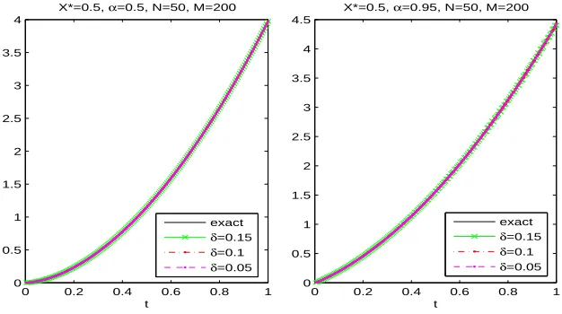
Example 2. Let the exact solution for problem (1)-(3) be u(x, t) =
t2sin(π
2x
)
. Therefore, ϕ(x) = u(x,0) = 0, k0(t) = u(0, t) = 0, k1(t) = u(1, t) = t2, f(x) = sin(π
2x
)
, and p(t) = 2 Γ(3−α)t
2−α+ π2
4 t
Galley
Pro
of
Using a LDG method for solving an inverse source problem ... 129 Table 1: Accuracy test for Example 1 for differentαwithx∗= 0.5.
N L2error Order L∞ error Order
α= 0.3 5 0.002067 - 0.002780 -10 0.000280 2.9 0.000376 2.9 15 0.000079 3.1 0.000112 3.0 20 0.000034 2.9 0.000047 3.0
α= 0.5 5 0.002068 - 0.002781 -10 0.000280 2.9 0.000376 2.9 15 0.000079 3.1 0.000112 3.0 20 0.000034 2.9 0.000047 3.0
α= 0.7 5 0.002069 - 0.002783 -10 0.000280 2.9 0.000377 2.9 15 0.000079 3.1 0.000112 3.0 20 0.000034 2.9 0.000047 3.0
α= 1 5 0.002070 - 0.002784 -10 0.000281 2.9 0.000377 2.9 15 0.000079 3.1 0.000112 3.0 20 0.000034 2.9 0.000047 3.0
x∗= 0.5, theng(t) = sin(π
4)t 2. pn
hforα= 0.5 andα= 0.95 with various noise
levelsδ= 5%, 10%, 15% are plotted in Fig. 3. Corresponding relative root mean square errors areε(p) = 8.5762×10⁻⁵, 8.6406×10⁻⁵, 8.7104×10⁻⁵
forα= 0.5 andε(p) = 2.030156×10⁻³, 3.077799×10⁻³, 4.153917×10⁻³for α= 0.95. In Table 2, we compare the relative root mean square errors for the
0 0.2 0.4 0.6 0.8 1
0 0.5 1 1.5 2 2.5 3 3.5 4
t
X*=0.5, α=0.5, N=50, M=200
exact δ=0.15
δ=0.1
δ=0.05
0 0.2 0.4 0.6 0.8 1
0 0.5 1 1.5 2 2.5 3 3.5 4 4.5
t
X*=0.5, α=0.95, N=50, M=200
exact δ=0.15
δ=0.1
δ=0.05
Galley
Pro
of
proposed method in [28] (ε1(p) for no regularization method and ε2(p) with
a regularization method) with the proposed LDG method (ε3(p)). In Table 3
the relative errors for differentx∗ withN= 50 are compared. The proposed method could generate more satisfactory results without any regularization method. To verify the role of the final time T, we depict pn
h for α= 0.95
withT = 100,10000 andδ= 5%, 10%, 15% in Fig. 4. We can see that the dependency of the results to final timeT is almost unimportant, even when
T is very large, i.e., T = 10000. Without any regularization method, the trace of the loss of stability does not appear.
Table 2: Comparison approximation solutions of Example 2 with the literature for various
α.
α= 0.1 α= 0.3 α= 0.5 α= 0.7 α= 0.9
δ= 5% ε1(p) 0.0773 0.0880 0.1230 0.2651 0.8079
ε2(p) 0.0331 0.0362 0.0393 0.0413 0.0431
ε3(p) 2.162×10⁻⁶ 1.9319×10⁻⁵ 8.5698×10⁻⁵ 3.33882×10⁻⁴ 0.001419157
δ= 10% ε1(p) 0.1545 0.1738 0.2436 0.5296 1.6159
ε2(p) 0.0634 0.0633 0.0662 0.0721 0.0812
ε3(p) 2.1600×10⁻⁶ 1.9334×10⁻⁵ 8.6232×10⁻⁵ 3.51023×10⁻⁴ 0.002105562
δ= 15% ε1(p) 0.2322 0.2611 0.3658 0.7948 2.4241
ε2(p) 0.0952 0.0943 0.0948 0.0721 0.1248
ε3(p) 2.1660×10⁻⁶ 1.9356×10⁻⁵ 8.6557×10⁻⁵ 3.96662×10⁻⁴ 0.002444287 Table 3: Comparison approximation solutions of Example 2 with the literature for various
x∗.
x∗ ε1(p) ε2(p) ε3(p)
0.1 1.0010 0.1801 1.024501×10⁻³
0.2 0.9047 0.0661 8.97953×10⁻⁴
0.3 0.9197 0.0767 8.03529×10⁻⁴
0.4 0.9323 0.0694 7.96885×10⁻⁴
0.5 0.9222 0.0839 7.50627×10⁻⁴
0.6 0.9071 0.0761 7.92723×10⁻⁴
0.7 0.9147 0.1026 7.78528×10⁻⁴
0.8 0.9256 0.0974 7.55676×10⁻⁴
Example 3. We test a none-smooth problem corresponding to (1)-(3), with
ϕ(x) =u(x,0) = sin(2πx),k0(t) =u(0, t) = 0,k1(t) =u(1, t) = 0,f(x) =x2,
and
p(t) =
{
2t+α, t∈[0,0.5],
Galley
Pro
of
Using a LDG method for solving an inverse source problem ... 131
0 20 40 60 80 100 0
0.5 1 1.5 2 2.5x 10
4
t exact
δ=0.15
δ=0.1
δ=0.05
0 2000 4000 6000 8000 10000 0
0.5 1 1.5 2 2.5x 10
8
t exact
δ=0.15
δ=0.1
δ=0.05
Figure 4: Numerical approximations topfor Example 2 forT = 100 (left) andT= 10000 (right).
Since the exact solution of this problem is not accessible, we first solve a direct problem using a suitable LDG method to obtain the input data g
then we solve the inverse problem using our method. In [28], the direct problem has been solved by using an implicit finite difference (FD) method but sincepis not a smooth function we expect to have a none-smooth solution and we decided to solve the direct problem using a LDG method too. We have to point out that since in our method we face the sparse systems, the computational complexity of both methods, i.e., FD and LDG is almost equal.
pn
h forα = 0.5, 0.95 with noise levels δ = 5%, 10%, 15% are presented in
Fig 5. Without applying any regularization methods, our results are in good agreement with the results of [28]. The corresponding relative root mean square errors are ε(p) = 3.8300×10⁻⁷, 6.2300×10⁻⁷, 9.4800×10⁻⁷ for α = 0.5 and ε(p) = 1.03320×10⁻⁴, 2.33279×10⁻⁴, 1.03320×10⁻⁴ for α= 0.95, which are considerably better than reported in [28].
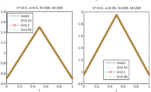
Example 4. We test a discontinuous problem corresponding to (1)-(3), with
ϕ(x) =u(x,0) = sin(2πx),k0(t) =u(0, t) = 0,k1(t) =u(1, t) = 0,f(x) =x2,
and
p(t) =
{
1, t∈[0.25,0.75],
0, t∈[0,0.25)∪(0.75,1].
Since the exact solution of this problem is not accessible, we first solve a direct problem using a suitable LDG method to obtain the input data g
Galley
Pro
of
0 0.2 0.4 0.6 0.8 1 0.4
0.6 0.8 1 1.2 1.4 1.6 1.8
t
X*=0.5, α=0.5, N=200, M=200
exact
δ=0.15
δ=0.1
δ=0.05
0 0.2 0.4 0.6 0.8 1 0.8
1 1.2 1.4 1.6 1.8 2
t
X*=0.5, α=0.95, N=200, M=200
exact
δ=0.15
δ=0.1
δ=0.05
Figure 5: Numerical approximations topfor Example 3 with variousα.
have to point out that since in our method we face the sparse systems, the computational complexity of both methods, i.e., FD and LDG is almost equal.
pn
h forα= 0.5, 0.95 with noise levels δ= 5%, 10%, 15% are plotted in Fig
6. Without applying any regularization methods, our results are in good agreement with the results of [28]. The corresponding relative root mean square errors are ε(p) = 4.1200×10⁻⁷, 6.2300×10⁻⁷, 8.2700×10⁻⁷ for α = 0.5 and ε(p) = 8.8388×10⁻⁵, 1.61535×10⁻⁴, 2.58527×10⁻⁴ for α= 0.95, which are considerably better than reported in [28].
0 0.2 0.4 0.6 0.8 1
−0.2 0 0.2 0.4 0.6 0.8 1 1.2
t
X*=0.5, α=0.5, N=200, M=200
exact δ=0.15
δ=0.1
δ=0.05
0 0.2 0.4 0.6 0.8 1
−0.2 0 0.2 0.4 0.6 0.8 1 1.2
t
X*=0.5, α=0.95, N=200, M=200
exact δ=0.15
δ=0.1
δ=0.05
Galley
Pro
of
Using a LDG method for solving an inverse source problem ... 133
5 Conclusion
In this paper, an inverse source problem for the time-fractional diffusion equa-tion was solved numerically by using a local discontinuous Galerkin method. In fact, we could extend a fully-discrete LDG finite element method for solv-ing a class of time-fractional inverse problem. By applysolv-ing this method with-out using any regularization methods, we could obtain stable and accurate numerical approximations to the time-dependent source term using an addi-tional data in an interior measurement location. The numerical stability and convergence of the proposed method have been investigated and theoretically proven. Various numerical examples with smooth or none-smooth data and maybe solutions have been verified to demonstrate the effectiveness and ro-bustness of the proposed method. This outstanding and promising method can be further applied to another one-dimensional or higher dimensional in-verse problems which can be considered for the future works.
References
1. Cheng, J., Nakagawa, J., Yamamoto, M. and Yamazaki, T. Uniqueness in an inverse problem for a one-dimensional fractional diffusion equation, Inverse Probl, 25 (11) (2009), 115002.
2. Cockburn, B., Kanschat, G., Perugia, I. and Schotzau, D. Superconver-gence of the local discontinuous Galerkin method for elliptic problems on cartesian grids, SIAM J. Numer. Anal, 39 (2001), 264-285.
3. Cockburn, B. and Shu, C.W. The Runge-Kutta discontinuous Galerkin method for conservation laws, V: multidimensional systems, J. Comput. Phys, 141 (1998), 199-224.
4. Cockburn, B. and Shu, C.W.The local discontinuous Galerkin method for time-dependent convection-diffusion systems, SIAM J. Numer. Anal, 35 (1998), 2440-2463.
5. Deng, W.H. Finite element method for the space and time fractional Fokker-Planck equation, SIAM J. Numer. Anal, 47 (2008), 204-226. 6. Deng, W.H. and Hesthaven, J.S.Local discontinuous Galerkin methods for
fractional diffusion equations, Math. Modelling Numer. Anal, 47 (2013), 1845-1864.
Galley
Pro
of
8. Dou, F.F. and Hon, Y.C. Numerical computation for backward time-fractional diffusion equation, Eng. Anal. Boundary Elem, 40 (2014), 138-146.
9. Jiang, Y.J. and Ma, J.T. High-order finite element methods for time-fractional partial differential equations, J. Comput. Appl. Math, 235 (2011), 3285-3290.
10. Jin, B.T. and Rundell, W. An inverse problem for a one-dimensional time-fractional diffusion problem, Inverse Probl, 28 (7) (2012), 075010. 11. Li, C.Z. and Chen, Y. Numerical approximation of nonlinear fractional
differential equations with subdiffusion and superdiffusion, Comput. Math. Appl, 62 (2011), 855-875.
12. Lin, Y.M. and Xu, C.J.Finite difference/spectral approximations for the time-fractional diffusion equation, J. Comput. Phys, 225 (2007), 1533-1552.
13. Liu, J.J. and Yamamoto, M.A backward problem for the time-fractional diffusion equation, Appl. Anal, 89 (2010), 1769-1788.
14. Liu, Y., Zhang, M., Li, H., Li, J.High-order local discontinuous Galerkin method combined with WSGD-approximation for a fractional subdiffusion equation, Comput. Math. Appl, 73 (2017), 1298-1314.
15. Metzler, R., Gl¨ockle, W.G. and Nonnenmacher, T.F. Fractional model equation for anomalous diffusion, Physica A, 211 (1994), 13-24.
16. Mohammadi, M., Mokhtari, R. and Panahipour, H.Solving two parabolic inverse problems with a nonlocal boundary condition in the reproducing kernel space, Appl. Comput. Math, 13 (2014), 91-106.
17. Mohammadi, M., Mokhtari, R. and Toutian, F.Solving an inverse prob-lem for a parabolic equation with a nonlocal boundary condition in the reproducing kernel space, Iranian J. Numer. Anal. Optimization, 4 (2014), 57-76.
18. Murio, D.A. Stable numerical solution of a fractional-diffusion inverse heat conduction problem, Comput. Math. Appl, 53 (2007), 1492-1501. 19. Murio, D.A. Time fractional IHCP with Caputo fractional derivatives,
Comput. Math. Appl, 56 (2008), 2371-2381.
20. Murio, D.A.Stable numerical evaluation of Gr¨unwald-Letnikov fractional derivatives applied to a fractional IHCP, Inverse Probl. Sci. Eng, 17 (2009), 229-243.
Galley
Pro
of
Using a LDG method for solving an inverse source problem ... 135 22. Qian, Z.Optimal modified method for a fractional-diffusion inverse heat
conduction problem, Inverse Probl. Sci. Eng, 18 (2010), 521-533.
23. Rashedi, K., Adibi, H., Dehghan. M. Determination of space-time-dependent heat source in a parabolic inverse problem via the Ritz-Galerkin technique, Inverse Probl. Sci. Eng, 22 (2014), 1077-1108.
24. Sakamoto, K. and Yamamoto, M.Initial value/boundary value problems for fractional diffusion-wave equations and applications to some inverse problems, J. Math. Anal. Appl, 382 (2011), 426-447.
25. Tuan, V.K.Inverse problem for fractional diffusion equation, Fractional Calculus Appl. Anal, 14 (2011), 31-55.
26. Wang, T., Wang, Y.M.A modified compact ADI method and its extrapola-tion for two-dimensional fracextrapola-tional subdiffusion equaextrapola-tions, J. Appl. Math. Comput, 52 (2016), 439-476.
27. Wei, T. and Wang, J.G. A modified quasi-boundary value method for an inverse source problem of the time-fractional diffusion equation, Appl. Numer. Math, 78 (2014), 95-111.
28. Wei, T. and Zhang, Z.Q.Reconstruction of a time-dependent source term in a time-fractional diffusion equation, Eng. Anal. Boundary Elem, 37 (2013), 23-31.
29. Wei, T., Zhang, Z.Q.Stable numerical solution to a Cauchy problem for a time fractional diffusion equation, Eng. Anal. Boundary Elem, 40 (2014), 128-137.
30. Xu, Q. and Hesthaven, J.S.Discontinuous Galerkin method for fractional convection-diffusion equations, To appear in SIAM J. Numer. Anal 31. Xu, Y. and Shu, C.W. Local Discontinuous Galerkin method for the
Camassa-Holm equation, 46 (2008), 1998-2021.
32. Yeganeh, S., Mokhtari, R., Hesthaven, J.S.Space-dependent source deter-mination in a time-fractional diffusion equation using a local discontinuous Galerkin method, BIT Numer Math, DOI 10.1007/s10543-017-0648-y. 33. Zhang, Y. and Xu, X. Inverse source problem for a fractional diffusion
equation, Inverse Probl, 27 (3) (2011), 035010.
34. Zheng, G.H. and Wei, T. Spectral regularization method for a Cauchy problem of the time fractional advection-dispersion equation, J. Comput. Appl. Math, 233 (2010), 2631-2640.
یدﻻﻮﻓ ﻪﻴﻤﺳ و یرﺎﺘﺨﻣ ﺎﺿر ،ﻪﻧﺎﮕﻳ ﻪﻴﻤﺳ
ﯽﺿﺎﯾر مﻮﻠﻋ هﺪﮑﺸﻧاد ،نﺎﻬﻔﺻا ﯽﺘﻌﻨﺻ هﺎﮕﺸﻧاد
١٣٩۵ ﺖﺸﻬﺒﯾدرا ٣ ﻪﻟﺎﻘﻣ شﺮﯾﺬﭘ ،١٣٩۶ ﻦﯾدروﺮﻓ ٩ هﺪﺷ حﻼﺻا ﻪﻟﺎﻘﻣ ﺖﻓﺎﯾرد ،١٣٩۵ ﻦﻤﻬﺑ ٣ ﻪﻟﺎﻘﻣ ﺖﻓﺎﯾرد
نوراو ﻞﺋﺎﺴﻣ ﯽﺧﺮﺑ ﻞﺣ یاﺮﺑ ار (LDG) ﯽﻌﺿﻮﻣ ﻪﺘﺳﻮﻴﭘﺎﻧ ﻦﻴﻛﺮﻟﺎﮔ شور ﻚﻳ ﻪﻟﺎﻘﻣ ﻦﻳا رد : هﺪﯿﮑﭼ
رﺎﺸﺘﻧا ﻪﻟدﺎﻌﻣ عﻮﻧ زا نوراو ﻪﻟﺎﺴﻣ ﻚﻳ رد ار نﺎﻣز ﻪﺑ ﻪﺘﺴﺑاو ﻊﺒﻨﻣ ﻪﻠﻤﺟ ﻊﻗاو رد .ﻢﻳﺮﺑ ﯽﻣ رﺎﻛ ﻪﺑ یﺮﺴﻛ (LDG) شور ﻚﻳ و نﺎﻣز رد ﯽﻫﺎﻨﺘﻣ ﻞﺿﺎﻔﺗ حﺮﻃ ﻚﻳ سﺎﺳا ﺮﺑ شور ﻦﻳا .ﻢﻴﻨﻛ ﯽﻣ ﻦﻴﻴﻌﺗ ﯽﻧﺎﻣز-یﺮﺴﻛ لﺎﺜﻣ ﺪﻨﭼ ،نﺎﻳﺎﭘ رد .دﻮﺷ ﯽﻣ ﺎﻴﻬﻣ ﺎﻄﺧ ﻦﻴﻤﺨﺗ ﻚﻳ هوﻼﻋ ﻪﺑ یدﺪﻋ یراﺪﯾﺎﭘ ﻪﯿﻀﻗ ﮏﯾ .ﺖﺳا نﺎﮑﻣ رد شور ﻪﻛ دﺮﻛ هرﺎﺷا ﺪﻳﺎﺑ .ﺪﻧﻮﺷ ﯽﻣ ﺶﻳﺎﻣزآ ،شور ﯽﺸﺨﺑﺮﺛا نداد نﺎﺸﻧ و یﺮﻈﻧ ﺞﻳﺎﺘﻧ ﺪﻴﺋﺎﺗ رﻮﻈﻨﻣ ﻪﺑ یدﺪﻋ نوراو ﻞﺋﺎﺴﻣ ﻦﻴﻨﭼ ﻞﺣ رد یدﺪﻋ یﺎﻫ شور ﺮﻳﺎﺳ یاﺮﺑ ﻪﻛ یزﺎﺳ ﻢﻈﻨﻣ یﺎﻬﺷور زا هدﺎﻔﺘﺳا نوﺪﺑ یدﺎﻬﻨﺸﻴﭘ .ﺪﻨﻛ ﯽﻣ ﺪﻴﻟﻮﺗ ار ﯽﻘﻴﻗد و راﺪﻳﺎﭘ یدﺪﻋ یﺎﻫ ﺐﻳﺮﻘﺗ ،ﺪﻨﺘﺴﻫ یروﺮﺿ حﺮﻃﺪﺑ