IJCSIT, Volume 2, Issue 5 (October, 2015) e-ISSN: 1694-2329 | p-ISSN: 1694-2345
COMPARISON OF CLASSIFICATION
ALGORITHMS AND DESIGN OF A
PERCENTAGE-SPLIT BASED METHOD
FOR DATA CLASSIFICATION
Niharika Chaudhary
1, Gaurav Mehta
2, Karan Bajaj
31, 2, 3Computer Science and Engineering Department, Chitkara University, Himachal Pradesh, India 1
[email protected], [email protected], 3
Abstract- Reliable data holds a lot of significance and is
needed in every field. The concept of data mining facilitates defect prediction and thus helps in achieving reliability of data with the use of various techniques and algorithms. Classification is an important data mining technique as it is widely used by researchers. Accurate assignment of class labels to data points is essential which can be achieved through classification. In this research, an evaluation of SMO, Random Forest and J48 classification algorithms is done based on application of these algorithms on the NASA defect data sets available from the PROMISE repository. The implementation of these algorithms is carried out on four data sets namely JM1, KC1, CM1 and PC1 along with a comparative study using Waikato Environment for Knowledge Analysis (WEKA) data mining tool. Performance measures such as Accuracy, Precision, Mean Absolute Error (MAE) and Root Mean Squared Error (RMSE) are used to examine the performance of these classifiers by making use of attribute selection methods and hence classification by cross-validation. Attribute selection of attributes is done before applying the classifiers so that only the most relevant attributes are taken into account. In addition to that, a different approach for classification (by using WEKA API) is built in Eclipse (Mars) SDK which produces an increase in the accuracy of classification of the selected data sets.
Index Terms- accuracy, classification, data mining, J48,
precision, Random Forest, SMO, WEKA
I. INTRODUCTION
Data mining is a rapidly growing discipline of computer science which is being employed in almost every field such as medicine, banking, intrusion detection, health care, transportation, etc. Amount of data is multiplying day by day and therefore, the need of the hour is to make this data reliable as well as manageable [1]. This can be achieved by proper inspection and cleaning of data with the use of attribute selection methods and data mining algorithms such as classification.
Attribute selection is applied in order to make the data set smaller in size by selection of the most important and relevant attributes. This leads to production of more efficient classification results as the non-relevant and noisy
attributes are discarded as they have negligible or no contribution in better classification [2].
Assigning class labels to data points known as classification is based on the approach that first it learns from a training set which contains already classified data points and then the built model is used to label new data points. SMO, J48 and one of the strongest classification algorithms Random Forest are analysed in this paper.
The aim of this paper is to evaluate the performance of the above mentioned classification algorithms and perform a comparative study with other research works. The implementation of these algorithms is carried out in WEKA data mining tool on JM1, CM1, KC1 and PC1 data sets freely available from the PROMISE data repository. Also, a method based on percentage split developed in Eclipse platform is presented.
The rest of this paper is presented as follows: in the next section we discuss related work in this area. In Section 3, a short description of the data sets and classifiers used is given. Section 4 throws light on the performance measures based on which these algorithms will be evaluated. In Section 5, results are documented and comparison of the results is done. Section 6 presents the designed methodology. Sections 7 and 8 conclude the paper and list the references respectively.
II. RELATEDWORK
Much research has been done in the field of defect prediction by classification algorithms. In [3], several data mining techniques in order to find the fault prone modules were discussed. Exploration of issues and problems faced in the area of defect prediction as well as solutions to improve product quality were identified in this paper. In addition to that, they also compared the data mining algorithms to find out the best algorithm for defect prediction. The conclusion that they drew was that the selection of a good data mining algorithm depends upon factors such as problem domain, types of data sets, nature of project, etc. Various fault prediction techniques like Decision Trees, Neural Networks, Density based clustering approach, Bagging method and Naïve Bayes were studied in [4]. They concluded that fault prediction is necessary to decrease the cost of testing and to improve reliability.
introduced the process of defect prediction and described the evaluation measures and the different defect prediction metrics for comparing the performance of data mining algorithms. Moreover, they also listed the challenging issues for defect prediction.
Comparative analysis among different algorithms has also been performed by researchers in this field. In [6], a hybrid approach for feature selection by using Filter and Wrapper feature selection techniques was introduced. Their study involved the use of KC1 NASA data set available from PROMISE repository. Firstly, the Filter methods such as OneR, GainRatio, ChiSquared, etc were used to select relevant features from the data set. Secondly, the optimal subset of features was obtained by applying Wrapper methods such as Naïve Bayes on the filtered features. The results obtained showed that the reduced feature subset gives better performance in terms of accuracy by the hybrid approach. Different feature selection algorithms such as PrincipalComponenets, GainRatio, FilteredAttributeEval and ReliefAttributeEval and classification algorithms such as SimpleCart, RandomTree, NaiveBayes, etc. for predicting the values of precision, recall, f-measure and accuracy on NASA PROMISE data sets CM1, JM1, PC1 and KC1 were used in [7]. She compared the results obtained by classification without feature selection with those obtained after applying feature selection algorithms and found out the best results among them. The conclusion drawn from her research was that in data sets CM1 and KC1, values of all four performance measures increased after selecting features by a ranker algorithm. JM1 data set showed higher values of recall and f-measure when feature selection was applied and data set PC1 produced improved values of recall, f-measure and accuracy. Highest accuracy obtained was 93.778% when feature selection was applied. A comparative performance analysis of various machine learning algorithms on publicly available NASA data sets was performed in [8]. A comparison was drawn on the basis of values of three performance measures i.e. accuracy, Mean Absolute Error (MAE) and F-measure. The best accuracy values were obtained by SVM, MLP and Bagging techniques on all the data sets. KNN performed poorly by showing lowest values of accuracy and F-measure and high values of MAE. Then, a new algorithm named “Improved Random Forest” was proposed in [2] which showed better accuracy than Random Forest. The best feature selection algorithm “Correlation based feature subset selection” was used to select six optimal features from four NASA PROMISE data sets PC1, PC2, PC3 and PC4 and then Random Forest classifier was applied. This method performed better than Random Forest in terms of accuracy.
III. DATASETSANDCLASSIFIERSUSED
In this paper, publicly available NASA defect data sets from the PROMISE data repository [9] have been used. These data sets are defect data from actual NASA projects. Table I provides information about the data sets which will be used to do experiments in this paper. This research work aims at applying attribute selection and classification algorithms to these data sets.
TABLE I DETAILS OFDATASETS Data Set Language
Number of attributes/ features
Number of instances
JM1 C 22 9593
KC1 C++ 22 2096
CM1 C 21 496
PC1 C 22 1107
The following classifiers are used in this research:
A. SMO
Proposed by John C. Platt in 1998, Sequential Minimal Optimization (SMO) algorithm breaks large data/problems into many smallest possible data/problems. It is simple and has the ability to handle very large data sets.
B. Random Forest
Developed by Leo Breiman and Adele Cutler, this classifier is a collection of many classification trees, hence known as a forest. The mode of the output classes of each classification tree is the overall output of Random Forest. Random Forest performs efficiently on large data sets. No pruning is done in the trees [10].
C. J48
A decision tree classifier which handles missing values very well. It is a widely used classifier in research areas. A tree is built which decides at each step that which node should be selected at each level.
IV. PERFORMANCEMEASURES
The performance of data mining algorithms can be evaluated based on some parameters or measures such as Accuracy, Precision, Mean Absolute Error (MAE) and Root Mean Squared Error (RMSE). These parameters help in estimating the level of correctness or how well the algorithm performs.
A. Confusion Matrix
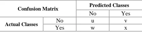
A confusion matrix or error matrix is a table that is used to visualize or describe a classifier’s performance [11]. It gives information about the correct and incorrect classifications made by a classifier against the actual outcomes (classes) in the data [12]. The rows represent actual classes while the columns represent predicted classes. The data in the matrix is used to evaluate the performance of classifiers. A confusion matrix is structured as shown in Table II.
TABLE III
A GENERALCONFUSIONMATRIX
Confusion Matrix Predicted Classes
No Yes
Actual Classes No u v
Yes w x
1) True Positives (TP): These are the number of predicted ‘yes’ classes that are actually ‘yes’ or the number of predicted ‘no’ classes that are actually ‘no’ [11].
2) False Positives (FP): These are the number of predicted ‘yes’ classes that are actually ‘no’ the number of predicted ‘no’ classes that are actually ‘yes’ [11].
3) False Negatives (FN): These are the number of defective classes that are incorrectly classified as non-defective.
4) True Negatives (TN): These are the number of non-defective classes that are correctly classified as non-defective.
The following performance measures are calculated from the confusion matrix:
1) Accuracy: The ratio of correctly identified defective classes to total number of classes.
= + ++ +
2) Precision:The proportion of predicted ‘yes’ or ‘no’ classes that are correct.
= +
3) Mean Absolute Error (MAE): MAE measures the deviation between predicted and actual output [13].
= 1/ ( − )
where, t = total number of instances po = predicted output eo = expected output
4) Root Mean Squared Error (RMSE):
= 1/ ( − )
Higher values of accuracy and precision but lower values of MAE and RMSE indicate better classification.
V. EXPERIMENTALWORKANDRESULTS
In this paper, we have performed implementation of classification algorithms on jm1.arff, kc1.arff, cm1.arff and pc1.arff data sets available from the PROMISE data repository [9]. The implementation and comparison is carried out in Waikato Environment for Knowledge Analysis (WEKA) [14], an open source data mining tool consisting of inbuilt algorithms. It was developed at the University of Waikato, New Zealand. . It is freely available under the GNU General Public License. The WEKA workbench contains a collection of visualization tools and algorithms for carrying out data analysis and predictions. The graphical user interface (GUI) makes it easier to carry out experimental work. The version of WEKA used in this study is WEKA 3.7.
The data sets are fed into the tool one by one and CfsSubsetEval, OneR attribute selection algorithms are applied on them. CfsSubsetEval uses BestFirst search method and displays a list of the best attributes which can
substantially contribute in better classification. Only these attributes are kept and the rest are removed from the data set. Then this reduced data set is classified by 10-fold cross validation application of classification algorithms mentioned in Section III. One Rule (or OneR) is a Ranker attribute selection method which displays the list of attributes based on their ranks in the selection process. Higher ranked attributes are selected for classification to produce better results.
TABLE IIIII
RESULTS OFDATASETSBASED ONACCURACY(%)
RF- Random Forest
Table III shows the values of accuracy when SMO, Random Forest and J48 classifiers are applied after selecting features according to CFS and OneR methods. The best results for accuracy that were obtained in [7] for the same data sets after attribute selection are as shown in Table IV. It can be seen that Random Forest gives higher accuracy as compared to SMO and J48 algorithms in Table III and the results shown in Table IV. Also, OneR is a better attribute selector as can be seen from Table III.
TABLE IVV
BESTRESULTSFORACCURACY(%) [7]
Data set Accuracy (%)
JM1 81.479
KC1 85.917
CM1 89.558
PC1 93.778
Fig. 1 Graph showing comparison between accuracy values of Table III and Table IV
Data set Attribute Selection-Classifier CFS-SMO OneR-SMO CFS-RF OneR -RF CFS-J48 OneR-J48 JM1
81.663 81.757 82.24
7 83.227 81.684 80.59
KC1
84.494 84.542 85.35
3 86.593 84.732 85.687
CM1
90.322 90.322 88.91
1 89.919 89.717 89.314 PC1
93.134 93.044 94.03
7 93.947 93.224 93.766 1) True Positives (TP): These are the number of
predicted ‘yes’ classes that are actually ‘yes’ or the number of predicted ‘no’ classes that are actually ‘no’ [11].
2) False Positives (FP): These are the number of predicted ‘yes’ classes that are actually ‘no’ the number of predicted ‘no’ classes that are actually ‘yes’ [11].
3) False Negatives (FN): These are the number of defective classes that are incorrectly classified as non-defective.
4) True Negatives (TN): These are the number of non-defective classes that are correctly classified as non-defective.
The following performance measures are calculated from the confusion matrix:
1) Accuracy: The ratio of correctly identified defective classes to total number of classes.
= + ++ +
2) Precision:The proportion of predicted ‘yes’ or ‘no’ classes that are correct.
= +
3) Mean Absolute Error (MAE): MAE measures the deviation between predicted and actual output [13].
= 1/ ( − )
where, t = total number of instances po = predicted output eo = expected output
4) Root Mean Squared Error (RMSE):
= 1/ ( − )
Higher values of accuracy and precision but lower values of MAE and RMSE indicate better classification.
V. EXPERIMENTALWORKANDRESULTS
In this paper, we have performed implementation of classification algorithms on jm1.arff, kc1.arff, cm1.arff and pc1.arff data sets available from the PROMISE data repository [9]. The implementation and comparison is carried out in Waikato Environment for Knowledge Analysis (WEKA) [14], an open source data mining tool consisting of inbuilt algorithms. It was developed at the University of Waikato, New Zealand. . It is freely available under the GNU General Public License. The WEKA workbench contains a collection of visualization tools and algorithms for carrying out data analysis and predictions. The graphical user interface (GUI) makes it easier to carry out experimental work. The version of WEKA used in this study is WEKA 3.7.
The data sets are fed into the tool one by one and CfsSubsetEval, OneR attribute selection algorithms are applied on them. CfsSubsetEval uses BestFirst search method and displays a list of the best attributes which can
substantially contribute in better classification. Only these attributes are kept and the rest are removed from the data set. Then this reduced data set is classified by 10-fold cross validation application of classification algorithms mentioned in Section III. One Rule (or OneR) is a Ranker attribute selection method which displays the list of attributes based on their ranks in the selection process. Higher ranked attributes are selected for classification to produce better results.
TABLE IIIII
RESULTS OFDATASETSBASED ONACCURACY(%)
RF- Random Forest
Table III shows the values of accuracy when SMO, Random Forest and J48 classifiers are applied after selecting features according to CFS and OneR methods. The best results for accuracy that were obtained in [7] for the same data sets after attribute selection are as shown in Table IV. It can be seen that Random Forest gives higher accuracy as compared to SMO and J48 algorithms in Table III and the results shown in Table IV. Also, OneR is a better attribute selector as can be seen from Table III.
TABLE IVV
BESTRESULTSFORACCURACY(%) [7]
Data set Accuracy (%)
JM1 81.479
KC1 85.917
CM1 89.558
PC1 93.778
Fig. 1 Graph showing comparison between accuracy values of Table III and Table IV
74 76 78 80 82 84 86 88 90 92 94 96 JM1 KC1 Accuracy (%) Data set Attribute Selection-Classifier CFS-SMO OneR-SMO CFS-RF OneR -RF CFS-J48 OneR-J48 JM1
81.663 81.757 82.24
7 83.227 81.684 80.59
KC1
84.494 84.542 85.35
3 86.593 84.732 85.687
CM1
90.322 90.322 88.91
1 89.919 89.717 89.314 PC1
93.134 93.044 94.03
7 93.947 93.224 93.766 1) True Positives (TP): These are the number of
predicted ‘yes’ classes that are actually ‘yes’ or the number of predicted ‘no’ classes that are actually ‘no’ [11].
2) False Positives (FP): These are the number of predicted ‘yes’ classes that are actually ‘no’ the number of predicted ‘no’ classes that are actually ‘yes’ [11].
3) False Negatives (FN): These are the number of defective classes that are incorrectly classified as non-defective.
4) True Negatives (TN): These are the number of non-defective classes that are correctly classified as non-defective.
The following performance measures are calculated from the confusion matrix:
1) Accuracy: The ratio of correctly identified defective classes to total number of classes.
= + ++ +
2) Precision:The proportion of predicted ‘yes’ or ‘no’ classes that are correct.
= +
3) Mean Absolute Error (MAE): MAE measures the deviation between predicted and actual output [13].
= 1/ ( − )
where, t = total number of instances po = predicted output eo = expected output
4) Root Mean Squared Error (RMSE):
= 1/ ( − )
Higher values of accuracy and precision but lower values of MAE and RMSE indicate better classification.
V. EXPERIMENTALWORKANDRESULTS
In this paper, we have performed implementation of classification algorithms on jm1.arff, kc1.arff, cm1.arff and pc1.arff data sets available from the PROMISE data repository [9]. The implementation and comparison is carried out in Waikato Environment for Knowledge Analysis (WEKA) [14], an open source data mining tool consisting of inbuilt algorithms. It was developed at the University of Waikato, New Zealand. . It is freely available under the GNU General Public License. The WEKA workbench contains a collection of visualization tools and algorithms for carrying out data analysis and predictions. The graphical user interface (GUI) makes it easier to carry out experimental work. The version of WEKA used in this study is WEKA 3.7.
The data sets are fed into the tool one by one and CfsSubsetEval, OneR attribute selection algorithms are applied on them. CfsSubsetEval uses BestFirst search method and displays a list of the best attributes which can
substantially contribute in better classification. Only these attributes are kept and the rest are removed from the data set. Then this reduced data set is classified by 10-fold cross validation application of classification algorithms mentioned in Section III. One Rule (or OneR) is a Ranker attribute selection method which displays the list of attributes based on their ranks in the selection process. Higher ranked attributes are selected for classification to produce better results.
TABLE IIIII
RESULTS OFDATASETSBASED ONACCURACY(%)
RF- Random Forest
Table III shows the values of accuracy when SMO, Random Forest and J48 classifiers are applied after selecting features according to CFS and OneR methods. The best results for accuracy that were obtained in [7] for the same data sets after attribute selection are as shown in Table IV. It can be seen that Random Forest gives higher accuracy as compared to SMO and J48 algorithms in Table III and the results shown in Table IV. Also, OneR is a better attribute selector as can be seen from Table III.
TABLE IVV
BESTRESULTSFORACCURACY(%) [7]
Data set Accuracy (%)
JM1 81.479
KC1 85.917
CM1 89.558
PC1 93.778
Fig. 1 Graph showing comparison between accuracy values of Table III and Table IV
KC1 CM1 PC1
Accuracy (%) Accuracy (%) [7] Data set Attribute Selection-Classifier CFS-SMO OneR-SMO CFS-RF OneR -RF CFS-J48 OneR-J48 JM1
81.663 81.757 82.24
7 83.227 81.684 80.59
KC1
84.494 84.542 85.35
3 86.593 84.732 85.687
CM1
90.322 90.322 88.91
1 89.919 89.717 89.314 PC1
93.134 93.044 94.03
TABLE V
RESULTS OFDATASETSBASED ONPRECISION
Table V shows that in terms of precision also the Random Forest algorithm performs better than the other two on an average and CFS and OneR perform equally well.
TABLE VI
RESULTS OFDATASETSBASED ONMAE
Lowest values of Mean Absolute Error (MAE) are obtained by SMO classifier and CFS attribute selector overall. For data set KC1, the lowest MAE value is 0.0687 which is better than that obtained in [6] i.e. 0.167.
TABLE VII
RESULTS OFDATASETSBASED ONRMSE
Random Forest classifier outputs lowest values of Root Mean Squared Error (RMSE) for all four data sets and CFS outperforms OneR yet again. Also, the best RMSE value for data set KC1 which is 0.2171 is better than the lowest value of 0.345 produced in [6].
Best results generated by this study are listed in Table VIII
TABLE VIII
BESTRESULTS
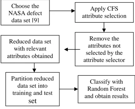
VI. DESIGNEDMETHODOLOGY FOR CLASSIFICATION
The best results produced by this study in the section above are the output of 10-fold cross validation technique in which the data set is divided into 10 partitions using each partition as a test set one by one. Here, a Random Forest classification based on percentage split criteria is shown which divides the data set into m: (n-m), where m is the size of training set and the remaining (n-m) is the size of
the test set, n being the total number of instances in the data set. This procedure has been designed in Eclipse (Mars) Software Development Kit (SDK) by incorporating the WEKA API.
Before the Random Forest classifier can be applied to the data set by percentage split criteria, CFS attribute selection is done because it showed better results than OneR. Attribute selection makes data less complex and redundancy is removed (if any).
Fig. 2 Flowchart of the proposed methodology
Algorithm (coded in Java using Eclipse (Mars) SDK):
Choose the data sets
Apply CFS attribute selection algorithm
Remove the unselected attributes from the data
If number of instances in data set is less than
1000, then split in the ratio 5:95 (where 5% is training set and 95% is test set)
Else split in the ratio 66:34 (where 66% is
training set and 34% is test set)
Apply Random Forest Classifier
Obtain Accuracy, Precision, MAE and RMSE values
5:95 split is done for CM1 data set as it has less than 1000 instances and other split ratios gave poorer results than the ones obtained by this ratio.
When this approach is implemented, results obtained which are shown in Table IX are better than our best results listed in Table VIII except for data set CM1.
TABLE IX
BESTRESULTS BYDESIGNEDMETHODOLOGY Data
set
Attribute Selection-Classifier
CFS-SMO
OneR -SMO
CFS-RF
OneR-RF
CFS-J48
OneR-J48 JM1 0.667 0.851 0.789 0.805 0.768 0.773 KC1 0.714 0.799 0.83 0.847 0.814 0.834 CM1 0.816 0.816 0.846 0.86 0.815 0.846 PC1 0.867 0.867 0.931 0.928 0.916 0.924
Data set
Attribute Selection-Classifier
CFS-SMO
OneR -SMO
CFS-RF
OneR-RF
CFS-J48
OneR -J48 JM1 0.1834 0.1824 0.2491 0.2469 0.2737 0.2553 KC1 0.1551 0.1546 0.1913 0.1881 0.222 0.2
CM1 0.0968 0.0968 0.1631 0.1602 0.174 0.166
PC1 0.0687 0.0696 0.0879 0.0957 0.1027 0.2434
Data set
Attribute Selection-Classifier
CFS-SMO
OneR -SMO
CFS-RF
OneR-RF
CFS-J48
OneR -J48 JM1 0.4282 0.4271 0.3623 0.3559 0.3738 0.3928 KC1 0.3938 0.3932 0.3233 0.3171 0.3488 0.3456 CM1 0.3111 0.3111 0.2941 0.2894 0.3056 0.3105 PC1 0.262 0.2637 0.2171 0.2238 0.2419 0.2434
Data
Set Accuracy (%) Precision MAE RMSE
JM1 83.227 0.851 0.1824 0.3559 KC1 86.593 0.847 0.1546 0.3171 CM1 90.322 0.86 0.0968 0.2894 PC1 94.037 0.931 0.0687 0.2171 Data
Set
Accuracy
(%) Precision MAE RMSE
JM1 87.9522 1 0.2439 0.341 KC1 92.9874 1 0.1538 0.2612 CM1 89.8089 0.807 0.1019 0.3192 PC1 98.6702 1 0.0392 0.1194
Choose the NASA defect
data set [9]
Apply CFS attribute selection
Remove the attributes not selected by the attribute selector Reduced data set
with relevant attributes obtained
Partition reduced data set into training and test
set
Fig. 3 Graph showing comparison between accuracy values of Table VIII and Table IX.
Fig. 4 Graph showing comparison between precision values of Table VIII and Table IX.
Fig. 5 Graph showing comparison between MAE values of Table VIII and Table IX.
Fig. 6 Graph showing comparison between RMSE values of Table VIII and Table IX.
VII. CONCLUSION ANDFUTUREWORK Defect prediction is a rapidly growing sub-field of data mining. Huge amount of data is produced everyday which should be cleaned. An important role of this research is that it has shown a new approach for data classification which reduces the data and hence classifies it with increased accuracy as well as reduced error. Four PROMISE data sets have been taken into account i.e. JM1, KC1, CM1 and PC1. They are fed into WEKA tool and combinations of attribute selectors and classifiers are employed on them by 10-fold cross validation method. The accuracy results thus obtained are better than those in [7] whereas the MAE and RMSE values show an improvement over the values produced in [6]. It can be seen that Random Forest algorithm outperforms SMO and J48.
The proposed approach which has been designed in Eclipse (Mars) SDK gives better values of performance measures accuracy, precision, MAE and RMSE for JM1, KC1 and PC1 data sets as compared to our previous results. This approach is based on Random Forest algorithm by performing 66:34 percentage split criteria for data sets having instances greater than 1000 and 5:95 ratio otherwise. These ratios give higher result values for accuracy and precision than cross-validation. Also, only the most relevant attributes are selected before classification.
Employing this approach on other data sets in the future to enhance the classification accuracy can be a good practice. In addition to that, other fields such as banking, medicine, etc. can also benefit from this methodology.
ACKNOWLEDGMENT
We are thankful to the PROMISE software engineering repository for providing free and easy access to the NASA defect data sets for use in our research.
REFERENCES
[1] N. Chaudhary, G. Mehta and K. Bajaj, “Data mining
methodologies to predict defects in data sets,”Advances in Computer Science and Information Technology (ACSIT),
vol. 2, no. 10, pp. 24-28, 2015.
[2] K. Magal and S. G. Jacob, “Improved random forest
algorithm for Software defect prediction through data 75
80 85 90 95 100
JM1 KC1 CM1
Accuracy % (by cross validation) Accuracy % (by percentage split)
0 0.2 0.4 0.6 0.8 1
JM1 KC1 CM1
Precision (by cross validation) Precision (by percentage split)
0 0.05 0.1 0.15 0.2 0.25
JM1 KC1 CM1
MAE (by cross validation) MAE (by percentage split)
Fig. 3 Graph showing comparison between accuracy values of Table VIII and Table IX.
Fig. 4 Graph showing comparison between precision values of Table VIII and Table IX.
Fig. 5 Graph showing comparison between MAE values of Table VIII and Table IX.
Fig. 6 Graph showing comparison between RMSE values of Table VIII and Table IX.
VII. CONCLUSION ANDFUTUREWORK Defect prediction is a rapidly growing sub-field of data mining. Huge amount of data is produced everyday which should be cleaned. An important role of this research is that it has shown a new approach for data classification which reduces the data and hence classifies it with increased accuracy as well as reduced error. Four PROMISE data sets have been taken into account i.e. JM1, KC1, CM1 and PC1. They are fed into WEKA tool and combinations of attribute selectors and classifiers are employed on them by 10-fold cross validation method. The accuracy results thus obtained are better than those in [7] whereas the MAE and RMSE values show an improvement over the values produced in [6]. It can be seen that Random Forest algorithm outperforms SMO and J48.
The proposed approach which has been designed in Eclipse (Mars) SDK gives better values of performance measures accuracy, precision, MAE and RMSE for JM1, KC1 and PC1 data sets as compared to our previous results. This approach is based on Random Forest algorithm by performing 66:34 percentage split criteria for data sets having instances greater than 1000 and 5:95 ratio otherwise. These ratios give higher result values for accuracy and precision than cross-validation. Also, only the most relevant attributes are selected before classification.
Employing this approach on other data sets in the future to enhance the classification accuracy can be a good practice. In addition to that, other fields such as banking, medicine, etc. can also benefit from this methodology.
ACKNOWLEDGMENT
We are thankful to the PROMISE software engineering repository for providing free and easy access to the NASA defect data sets for use in our research.
REFERENCES
[1] N. Chaudhary, G. Mehta and K. Bajaj, “Data mining
methodologies to predict defects in data sets,”Advances in Computer Science and Information Technology (ACSIT),
vol. 2, no. 10, pp. 24-28, 2015.
[2] K. Magal and S. G. Jacob, “Improved random forest
algorithm for Software defect prediction through data
CM1 PC1
Accuracy % (by cross validation) Accuracy % (by percentage split)
PC1 Precision (by cross validation) Precision (by percentage split)
CM1 PC1
MAE (by cross validation) MAE (by percentage split)
0 0.05 0.1 0.15 0.2 0.25 0.3 0.35 0.4
JM1 KC1
RMSE (by cross validation) RMSE (by percentage split)
Fig. 3 Graph showing comparison between accuracy values of Table VIII and Table IX.
Fig. 4 Graph showing comparison between precision values of Table VIII and Table IX.
Fig. 5 Graph showing comparison between MAE values of Table VIII and Table IX.
Fig. 6 Graph showing comparison between RMSE values of Table VIII and Table IX.
VII. CONCLUSION ANDFUTUREWORK Defect prediction is a rapidly growing sub-field of data mining. Huge amount of data is produced everyday which should be cleaned. An important role of this research is that it has shown a new approach for data classification which reduces the data and hence classifies it with increased accuracy as well as reduced error. Four PROMISE data sets have been taken into account i.e. JM1, KC1, CM1 and PC1. They are fed into WEKA tool and combinations of attribute selectors and classifiers are employed on them by 10-fold cross validation method. The accuracy results thus obtained are better than those in [7] whereas the MAE and RMSE values show an improvement over the values produced in [6]. It can be seen that Random Forest algorithm outperforms SMO and J48.
The proposed approach which has been designed in Eclipse (Mars) SDK gives better values of performance measures accuracy, precision, MAE and RMSE for JM1, KC1 and PC1 data sets as compared to our previous results. This approach is based on Random Forest algorithm by performing 66:34 percentage split criteria for data sets having instances greater than 1000 and 5:95 ratio otherwise. These ratios give higher result values for accuracy and precision than cross-validation. Also, only the most relevant attributes are selected before classification.
Employing this approach on other data sets in the future to enhance the classification accuracy can be a good practice. In addition to that, other fields such as banking, medicine, etc. can also benefit from this methodology.
ACKNOWLEDGMENT
We are thankful to the PROMISE software engineering repository for providing free and easy access to the NASA defect data sets for use in our research.
REFERENCES
[1] N. Chaudhary, G. Mehta and K. Bajaj, “Data mining
methodologies to predict defects in data sets,”Advances in Computer Science and Information Technology (ACSIT),
vol. 2, no. 10, pp. 24-28, 2015.
[2] K. Magal and S. G. Jacob, “Improved random forest
algorithm for Software defect prediction through data
KC1 CM1 PC1
mining techniques,” International Journal of Computer Application, vol. 117, no. 23, pp. 18-22, 2015.
[3] N. Azeem and S. Usmani, “Analysis of data mining based software defect prediction techniques,” Global Journal of Computer Science and Technology, vol. 11, 2011.
[4] A. Sanyaland B. Singh, “A systematic literature survey on various techniques for software fault prediction,” International Journal of Advanced Research in Computer Science and Software Engineering, vol. 4, pp. 1210-1212,
2014.
[5] N. Azeem and S. Usmani, “Defect prediction leads to high
quality product,” Journal of Software Engineering and Applications, vol. 4, pp. 639-645, 2011.
[6] C. A. Devi, K. E. Kannammal and B. Surendiran, “A hybrid feature selection model for software fault prediction,” International Journal on Computational Sciences and Applications, vol. 2, no. 2, pp. 25-35, 2012.
[7] V. Kaur, “Fault prediction in software modules using feature selection and machine learning methods,” International Journal of Scientific and Engineering Research, vol. 4, pp. 406-409, 2013.
[8] S. Aleem, L. F. Capretz and F. Ahmed, “Comparative
performance analysis of machine learning techniques for
software bug detection,”Computer Science and Information Technology (CS & IT-CSCP 2015), pp. 71-79, 2015.
[9] Software Defect Dataset, PROMISE REPOSITORY, http://promise.site.uottawa.ca/SERepository/datasets-page.html
[10] www.datasciencecentral.com/m/blogspot?id=6448529%3A BlogPost%3A106993
[11] http://www.dataschool.io/simple-guide-to-confusion-matrix-terminology/
[12] http://www.saedsayad.com/model_evaluation_c.htm [13] V. Jayaraj and N. S. Raman, “Software defect prediction
using boosting techniques,” International Journal of Computer Applications, vol. 65, no. 13, pp. 1-4, 2013.