NTNUSentEval at SemEval 2016 Task 4: Combining General Classifiers for Fast Twitter Sentiment Analysis

NTNUSentEval at SemEval-2016 Task 4:

Combining General Classifiers for Fast Twitter Sentiment Analysis

Brage Ekroll Jahren Valerij Fredriksen Bj¨orn Gamb¨ack Lars Bungum Department of Computer and Information Science

Norwegian University of Science and Technology (NTNU) Sem Sælands vei 7–9, NO–7491 Trondheim, Norway

{brageej,valerijf_}@stud.ntnu.no _{gamback,larsbun_}@idi.ntnu.no

Abstract

The paper describes experiments on sentiment classification of microblog messages using an architecture allowing general machine learn-ing classifiers to be combined either sequen-tially to form a multi-step classifier, or in par-allel, creating an ensemble classifier. The sys-tem achieved very competitive results in the shared task on sentiment analysis in Twitter, in particular on non-Twitter social media data, that is, input it was not specifically tailored to.

1 Introduction

As a growing platform for people to express them-selves on a global scale, Twitter has become exceed-ingly attractive as an information source. In addi-tion to text, a tweet comes with metadata such as the sender’s location and language, and hashtags, mak-ing it possible to quickly gather vast amounts of data regarding a specific product, person or event. With a working Twitter Sentiment Analysis system, compa-nies could get a feel of what consumers think of their products, or politicians could estimate their popular-ity amongst Twitter users in specific regions.

However, tweets and other informal texts on so-cial media are quite different from texts elsewhere. They are short in length and contain a lot of abbre-viations, misspellings, Internet slang, and creative syntax. Although the relative occurrence of non-standard English syntax is fairly constant among many types of social media (Baldwin et al., 2013),

∗_{Thanks to Mikael Brevik, Jørgen Faret, Johan Reitan and}

Øyvind Selmer for their work on two previous NTNU systems.

analysing such texts using traditional language pro-cessing systems can be problematic, primarily since the main common denominator of social media text is not that it is informal, but that it describes language in rapid change (Androutsopoulos, 2011; Eisenstein, 2013), so that resources targeted directly at social media language quickly become outdated.

Twitter Sentiment Analysis (TSA) has been a rapibly growing research area in recent years, and a typical approach to TSA has been identified, using a supervised machine learning strategy, consisting of three main steps: preprocessing, feature extraction and classifier training. Preprocessing is used in order to remove noise and standardize the tweet format, for example, by replacing or removing URLs. De-sired features of the tweets are then extracted, such as sentiment scores using specific sentiment lexica or the occurrence of different emoticons. Finally, a classifier is trained on the extracted features.

Since the machine learning algorithms used com-monly are supervised, sentiment-annotated data is a prerequisite for training — and the growth of the TSA research field can largely be attributed to the In-ternational Workshop on Semantic Evaluation (Sem-Eval) having run shared tasks on this theme since 2013 (Wilson et al., 2013), annually producing new annotated data. The SemEval-2016 version (Task 4) of the TSA task and the data sets are described by Nakov et al. (2016). Here we will specifically ad-dress Subtask A, which is a 3-way sentiment polar-ity classification problem, attributing the labels ‘pos-itive’, ‘negative’ or ‘neutral’ to tweets.

The rest of the paper is laid out as follows: Sec-tion 2 describes a general architecture for building

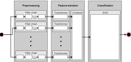
Figure 1: Overview of the core system architecture

Twitter sentiment classifiers, drawing on the expe-riences of developing two previous TSA systems (Selmer et al., 2013; Reitan et al., 2015). Section 3 reports the application of such a system (‘NTNU-SentEval’) to the SemEval data sets, while Section 4 points to ways that the results could be improved.

2 Sentiment Classifier Architecture

To solve the three-way sentiment classification task, a general multi-class classifier, BaseClassifier, was created. Utilizing a general methodology enables the combination of several BaseClassifiers in vari-ous ways, either sequentially to create a multi-step classifier, or in parallel, as a classifier ensemble.

The BaseClassifier consists of three steps: pre-processing, feature extraction, and then either classi-fication or training. These are handled by a Pipeline object built in the Scikit-Learn Python machine learning library (Pedregosa et al., 2011). Scikit-Learn Transformer objects are used to extract or generate feature representations of the data. Fig-ure 1 illustrates the overall architectFig-ure of the sys-tem. When creating a BaseClassifier instance, a set of parameters is specified, including the classifica-tion algorithm, the preprocessing funcclassifica-tions to use, and options for each of the transformers. The pre-processing methods invoked depend on the trans-formers and the features they aim to extract.

2.1 Preprocessing

The preprocessing step modifies the raw tweets be-fore they are passed to feature extraction: noise is fil-tered out and negation scope is detected. The filter-ing consists of a chain of simple methods usfilter-ing regu-lar expressions. There are ten basic filters that can be invoked, six of which replace various twitter-specific objects with the empty string: emoticons, username

mentions, RT (retweet) tags, URLs, only hashtag signs (#), and hashtags (incl. the string following the sign). The other four filters transform uppercase characters to lowercase, remove non-alphabetic or space characters, limit the maximum repetitions of a single character to three, and perform tokenization using Pott’s tweet tokenizer (Potts, 2011).

Negation detection uses a simple approach where nwords appearing after a negation cue, but before the next punctuation mark, are marked as negated. The negation cues were adopted from Councill et al. (2010), supplemented by five common mis-spellings obtained by looking up each negation cue in TweetNLP’s Twitter word cluster (Owoputi et al., 2013):anit,couldnt,dnt,does’nt, andwont.

2.2 Feature Extraction

The feature extraction is implemented as a Scikit-Learn Feature Union, which is a collection of inde-pendent transformers (feature extractors), that build a feature matrix for the classifier. Each feature is represented by a transformer. Eight such trans-formers have been implemented: two extract the number of punctuations(repeated alphabetical and grammatical signs) and the number of happy and sademoticonsfound in the tweet. Two other trans-formers extract TF–IDF values for word n-grams

andcharacter n-gramsusing a bag-of-words vector-izer implementation, which is an extension of Scikit-Learn’s defaultTfidfVectorizer.

A part-of-speech transformer uses the GATE TwitIE tagger (Derczynski et al., 2013) to assign part-of-speech tags to every token in the text; the tag occurrences are then counted and returned. Aword clustertransformer counts the occurrences of differ-ent TweetNLP word clusters (Owoputi et al., 2013), that is, if a word in a tweet is a member of a cluster, a counter for that specific cluster is incremented.

automatically annotated lexica used are NRC Senti-ment140 and HashtagSentiment (Kiritchenko et al., 2014), that contain sentiment scores for both uni-grams and biuni-grams, where some are in a negated context. Similarly, two manually annotated lexica, AFINN (Nielsen, 2011) and NRC Emoticon (Mo-hammad and Turney, 2010), give a sentiment score for each word (AFINN) or each emoticon (NRC Emoticon). However, two further manually anno-tated lexica, MPQA (Wilson et al., 2005) and Bing Liu (Ding et al., 2008), do not list sentiment scores for words, but only whether a word contains positive or negative sentiment. For those two lexica, nega-tive and posinega-tive word sentiments were mapped to the scores−1or+1, respectively.

For all lexica, four different features were ex-tracted from each tweet. Following Kiritchenko et al. (2014), the four features for manually annotated lexica are the sums of positive scores and of nega-tive scores for words in both affirmanega-tive and negated contexts, while the four features for automatically annotated lexica comprise the number of unigrams or bigrams with sentiment score6= 0, the sum of all sentiment scores, the highest sentiment score, and the score of the last unigram or bigram in the tweet.

2.3 Classification

After all desired features have been extracted, a BaseClassifier instance allows for the use of state-of-the-art classification algorithms such as Support Vector Machines (SVM), Na¨ıve Bayes and Maxi-mum Entropy (MaxEnt). Scikit-Learn includes a se-ries of implementations of the SVM algorithm (Vap-nik, 1995). The NTNUSentEval system uses the SVC variant, also known as C-Support SVM classi-fier since it is based on the idea of setting a constant C to penalize incorrectly classified instances. High C values create a narrower margin, enabling more elements to be correctly classified. However, this can lead to overfitting, so it is desirable to perform some kind of parameter optimization to find the best Cvalue. For multi-class classification, Scikit-Learn uses a One-vs-One method with a run time com-plexity more than quadratic to the number of ele-ments; however, this is not a problem for our rela-tively small (under 10,000 elements) datasets.

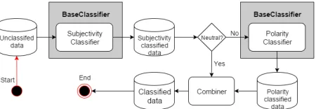
A single BaseClassifier acts as a one-step clas-sifier, but by chaining BaseClassifiers sequentially,

Figure 2: Data flow in the two-step classifier

a multi-step classifier can be created. Each classi-fier can be trained independently on different data, thereby learning a different classification function. Figure 2 illustrates how chaining two BaseClassi-fiers can create a two-step classifier. The first Base-Classifier is trained only on data labeled as subjec-tive or objecsubjec-tive, while the second BaseClassifier is trained only on subjective data, labeled positive or negative. When classifying, if the first Base-Classifier classifies an instance as subjective, the in-stance is forwarded to the second BaseClassifier to determine if it is positive or negative. The results from both classifiers are then combined and the final classification is returned.

By combining BaseClassifiers in parallel, an en-semble of classifiers can be created. Each of the classifiers is independent of the others and all clas-sify the same instances. In the end, the classifiers vote to decide on the classification of an instance. Since the BaseClassifiers are so general, it is pos-sible to create BaseClassifiers that extract different features, do different preprocessing, or use different classification algorithms — and then combine these to create an ensemble system.

2.4 Parameter Optimization

Feature tok

enize

lo

wer

case

no

emotes

no

user

no

rt

tag

no

url

no

hashsign

no

hashtag

limit

chars

limit

repeat

Wordn-grams X X X X X

Charn-grams X X X X X X

Lexicon X X X X X X X

PoS Tagger X X X X X

Word Clusters X X X X X X

Punctuation X X

Emoticons X

VADER X X X X

Table 1: Preprocessing used by feature extractors

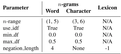
Parameter _{Word Character}n-grams Lexicon

n-range (1, 5) (3, 6) N/A

use idf True True N/A

min df 0.0 0.0 N/A

max df 0.5 0.5 N/A

negation length 4 None -1

Table 2: Optimal parameter settings

As described in Section 2.2, a total of eight dif-ferent feature extractors have been implemented, all of which can be enabled or disabled. Each feature extractor utilizes a specific preprocessor setting, as shown in Table 1. Further, there are three option settings for the SVM algorithm: type, kernel and C, which after grid search were set to SVC, Linear, and0.1, respectively. In addition to the preproces-sor options, there are eleven more feature extractor options, whose grid-searched optimal values are dis-played in Table 2, wheren-rangegives the lower and upper n-gram sizes,use idf enables Inverse Docu-ment Frequency weighting,min df andmax df give the proportions of lowest resp. highest document frequency occurring terms to be excluded from the final vocabulary, andnegation lengththe maximum number of tokens inside a negation scope.

3 Experimental Results

The NTNUSentEval TSA system was trained on the Twitter training set (8,748 tweets), using the opti-mal parameters identified through grid search, and tested on the SemEval Twitter test sets from 2013 and 2014. The complete results on these test sets are shown in Table 4 below, while Nakov et al. (2016)

give the results on all test sets, including the un-known 2016 tweet set, in terms of the official eval-uation metric, FPN

1 , which is the average of the F1-scores on the negative and the positive tweets.

Notably, our system performed extremely well on the out-of-domain test sets (i.e., the non-Twitter data), being the best of all 34 participating systems on the 2013-SMS set (with a0.641FPN

1 score, com-pared to a0.190FPN₁ baseline), the 3rd on the 2014-Live-journal set (FPN

1 = 0.719, with a 0.272 base-line), and overall tied for first on the out-of-domain data, supporting our claim that the approach taken in itself is quite general. However, the lack of do-main fine-tuning of the system showed in compar-ison to the best systems on Twitter data, with the NTNUSentEval system consistently placing 11–13 on the different test sets, including 11th on the 2016 set (FPN

1 = 0.583, with baseline0.255).

3.1 Ablation Study

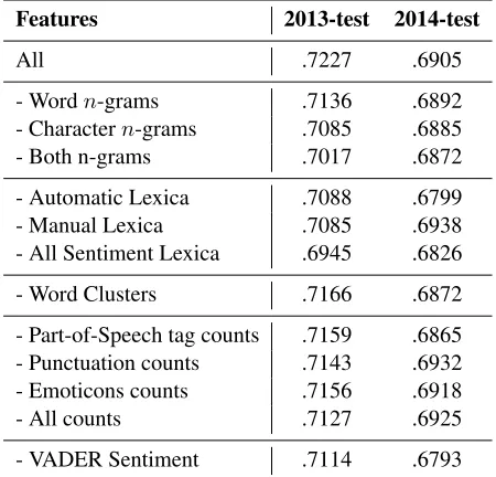
In order to detect the overall importance or impact each feature has, a simple ablation study was con-ducted by removing each feature in turn and check-ing how the performance of the system was affected. The results of this study are shown in Table 3.

Evidently, the single most important feature is Sentiment Lexica. On the 2013-test set, system ac-curacy is reduced from 0.7227 to 0.6945 when the feature is removed, while the effect of removing it when testing on the 2014 set is not as apparent. A possible reason for this difference may be that most of the sentiment lexica used were created at the same time as the 2013-test set, and they might thus better reflect the language in that period of time. As noted in Section 1, the language of social media is rapidly changing, so that a lexicon created in 2013 might have reduced value already for data collected a year later. This effect is also noticable when testing the system on the 2014-test set, where the VADER Sen-timent feature is the most important one, reducing the accuracy from 0.6905 to 0.6793 when being re-moved. On the 2013-test set, the VADER Sentiment feature, which was created in 2014, does not have the same impact, again indicating a change in how the language is used and that VADER might better reflect the Twitter language of 2014.

char-Features 2013-test 2014-test

All .7227 .6905

- Wordn-grams .7136 .6892

- Charactern-grams .7085 .6885

- Both n-grams .7017 .6872

- Automatic Lexica .7088 .6799

- Manual Lexica .7085 .6938

- All Sentiment Lexica .6945 .6826

- Word Clusters .7166 .6872

- Part-of-Speech tag counts .7159 .6865 - Punctuation counts .7143 .6932 - Emoticons counts .7156 .6918

- All counts .7127 .6925

- VADER Sentiment .7114 .6793

Table 3: Feature ablation study results (F1-scores)

acter n-grams and word n-grams lead to a degrada-tion in performance. On the 2013-test set the degra-dation in performance is quite significant, while on the 2014-test set the degradation is more subtle.

Another interesting result is the impact of the Emoticons and Punctuation count features. On the 2013-test set, removing them gives a slight reduction in performance, while on the 2014-test set we can observe a slightincreasein performance. One pos-sible reason for this could be that the way emoticons and punctuation are used in tweets changes over time, but the most likely cause is merely noise in the data. Although causing slightly increased or de-creased performance, the individual count features do not significantly affect the overall results.

3.2 Architectural Experiments

Two instances of the BaseClassifier can be chained sequentially creating a 2-step classifier. Such a clas-sifier was tested on the 2013 and 2014 test sets, as shown in Table 4. The 2-step classifier performs worse than the 1-step classifier on the 2013 set, while their performances on the 2014 set are com-parable, so based on these results it is not clear that 1-step classification is better than 2-step.

The GATE TwitIE part-of-speech tagger uses an underlying model when tagging tweets. In addition to the standard best performing model, another high-speed model trading 2.5% token accuracy for half

Data Precision Recall F1 Accuracy Time 1-step classifier

2013 .7370 .6639 .6848 .7227 106.97 2014 .7031 .6619 .6691 .6905 53.01

2-step classifier

2013 .7278 .6526 .6729 .7172 118.36 2014 .7079 .6570 .6676 .6912 59.6

1-step classifier with fast PoS tagging 2013 .7364 .6639 .6846 .7221 80.13 2014 .7032 .6591 .6673 .6892 41.03

Table 4: Sentiment classifier performance

the tagging speed is available, and the results from testing BaseClassifier using the high-speed tagger model are also shown in Table 4. Although a slight reduction in performance can be observed compared to using the best tagger model, the high-speed model significantly reduced the total execution time, from 107 to 80 seconds on the 2013-test set and from 53 to 41 seconds on the 2014-test set.

4 Conclusion and Future Work

Drawing on the experiences from two previous Twit-ter Sentiment Analysis systems (Selmer et al., 2013; Reitan et al., 2015), a new TSA system was created using a simplified and generalised architecture, al-lowing for accurate and fast tweet classification.

As seen in the ablation study of Section 3.1, the Sentiment Lexica is the single most important fea-ture, while also being one of the simplest: our im-plementation is based only on summing up the sen-timent value of each word. A possible improvement would thus be to extract more information by con-sidering the order of the words, part-of-speech tags, and degree modifiers, such as ‘very’, ‘really’ and ‘somewhat’, that can affect the sentiment value of the following word. These modifiers are currently not handled by the Sentiment Lexica extractor, yet they clearly carry a lot of sentiment weight.

References

Jannis Androutsopoulos. 2011. Language change and digital media: a review of conceptions and evidence. In Kristiansen and Coupland, editors, Standard Lan-guages and Language Standards in a Changing Eu-rope, pages 145–159. Novus, Oslo, Norway, February. Timothy Baldwin, Paul Cook, Marco Lui, Andrew MacKinlay, and Li Wang. 2013. How noisy social media text, how diffrnt social media sources? In6th International Joint Conference on Natural Language Processing, pages 356–364, Nagoya, Japan, October. Isaac G. Councill, Ryan McDonald, and Leonid

Ve-likovich. 2010. What’s great and what’s not: learning to classify the scope of negation for improved senti-ment analysis. In48th Annual Meeting of the Associa-tion for ComputaAssocia-tional Linguistics, pages 51–59, Up-psala, Sweden, July. ACL. Workshop on Negation and Speculation in Natural Language Processing.

Leon Derczynski, Alan Ritter, Sam Clark, and Kalina Bontcheva. 2013. Twitter part-of-speech tagging for all: Overcoming sparse and noisy data. In9th Interna-tional Conference on Recent Advances in Natural Lan-guage Processing, pages 198–206, Hissar, Bulgaria, September.

Xiaowen Ding, Bing Liu, and Philip S. Yu. 2008. A holistic lexicon-based approach to opinion mining. In

2008 International Conference on Web Search and Data Mining, pages 231–240, Stanford, California, February. ACM.

Jacob Eisenstein. 2013. What to do about bad language on the internet. In2013 Conference of the North Amer-ican Chapter of the Association for Computational Linguistics, pages 359–369, Atlanta, Georgia, June. C.J. Hutto and Eric Gilbert. 2014. VADER: A

parsimo-nious rule-based model for sentiment analysis of social media text. In 8th International Conference on We-blogs and Social Media, Ann Arbor, Michigan, June. Svetlana Kiritchenko, Xiaodan Zhu, and Saif M.

Mo-hammad. 2014. Sentiment analysis of short infor-mal texts. Journal of Artificial Intelligence Research, 50:723–762, August.

Saif Mohammad and Peter Turney. 2010. Emotions evoked by common words and phrases: Using Me-chanical Turk to create an emotion lexicon. In2010 Conference of the North American Chapter of the As-sociation for Computational Linguistics, pages 26–34, Los Angeles, California, June. ACL. Workshop on Computational Approaches to Analysis and Genera-tion of EmoGenera-tion in Text.

Preslav Nakov, Alan Ritter, Sara Rosenthal, Fabrizio Se-bastiani, and Veselin Stoyanov. 2016. SemEval-2016 Task 4: Sentiment analysis in Twitter. In10th Interna-tional Workshop on Semantic Evaluation, San Diego, California, June. ACL.

Finn ˚Arup Nielsen. 2011. A new ANEW: Evalu-ation of a word list for sentiment analysis in mi-croblogs. In1st Workshop on Making Sense of Micro-posts (#MSM2011), pages 93–98, Heraklion, Greece, May.

Olutobi Owoputi, Brendan O’Connor, Chris Dyer, Kevin Gimpel, Nathan Schneider, and Noah A. Smith. 2013. Improved part-of-speech tagging for online conversa-tional text with word clusters. In 2013 Conference of the North American Chapter of the Association for Computational Linguistics, pages 380–390, Atlanta, Georgia, June. ACL.

Fabian Pedregosa, Ga¨el Varoquaux, Alexandre Gram-fort, Vincent Michel, Bertrand Thirion, Olivier Grisel, Mathieu Blondel, Peter Prettenhofer, Ron Weiss, Vin-cent Dubourg, Jake Vanderplas, Alexandre Passos, David Cournapeau, Matthieu Brucher, Matthieu Per-rot, and ´Edouard Duchesnay. 2011. Scikit-learn: Ma-chine learning in Python. Journal of Machine Learn-ing Research, 12(1):2825–2830.

Christopher Potts. 2011. Sentiment symposium tutorial. InSentiment Analysis Symposium, San Francisco, Cal-ifornia, November. Alta Plana Corporation.

sentiment.christopherpotts.net/

Johan Reitan, Jørgen Faret, Bj¨orn Gamb¨ack, and Lars Bungum. 2015. Negation scope detection for Twitter sentiment analysis. In2015 Conference on Empirical Methods in Natural Language Processing, pages 99– 108, Lisbon, Portugal, September. 6th Workshop on Computational Approaches to Subjectivity, Sentiment and Social Media Analysis.

Øyvind Selmer, Mikael Brevik, Bj¨orn Gamb¨ack, and Lars Bungum. 2013. NTNU: Domain semi-independent short message sentiment classification. In

2nd Joint Conference on Lexical and Computational Semantics (*SEM), Vol. 2: 7th International Work-shop on Semantic Evaluation, pages 430–437, Atlanta, Georgia, June. ACL.

Vladimir N. Vapnik. 1995. The Nature of Statistical Learning Theory. Springer, New York, New York. Theresa Wilson, Paul Hoffmann, Swapna

Somasun-daran, Jason Kessler, Janyce Wiebe, Yejin Choi, Claire Cardie, Ellen Riloff, and Siddharth Patwardhan. 2005. OpinionFinder: A system for subjectivity analysis. In

2005 Human Language Technology Conference and Conference on Empirical Methods in Natural Lan-guage Processing, pages 34–35, Vancouver, British Columbia, October. ACL. Demonstration Abstracts. Theresa Wilson, Zornitsa Kozareva, Preslav Nakov, Alan