Proceedings of SemEval-2016, pages 1–18,
SemEval-2016 Task 4: Sentiment Analysis in Twitter
Preslav Nakov♣, Alan Ritter♦, Sara Rosenthal♥, Fabrizio Sebastiani♣∗, Veselin Stoyanov♠
♣Qatar Computing Research Institute, Hamad bin Khalifa University, Qatar ♦Department of Computer Science and Engineering, The Ohio State University, USA
♥IBM Watson Health Research, USA ♠Johns Hopkins University, USA
Abstract
This paper discusses the fourth year of the ”Sentiment Analysis in Twitter Task”. SemEval-2016 Task 4 comprises five sub-tasks, three of which represent a significant departure from previous editions. The first two subtasks are reruns from prior years and ask to predict the overall sentiment, and the sentiment towards a topic in a tweet. The three new subtasks focus on two variants of the basic “sentiment classification in Twitter” task. The first variant adopts a five-point scale, which confers anordinalcharacter to the clas-sification task. The second variant focuses on the correct estimation of the prevalence of each class of interest, a task which has been calledquantificationin the supervised learn-ing literature. The task continues to be very popular, attracting a total of 43 teams.
1 Introduction
Sentiment classification is the task of detecting whether a textual item (e.g., a product review, a blog post, an editorial, etc.) expresses a POSI -TIVE or a NEGATIVE opinion in general or about a given entity, e.g., a product, a person, a political party, or a policy. Sentiment classification has be-come a ubiquitous enabling technology in the Twit-tersphere. Classifying tweets according to sentiment has many applications in political science, social sci-ences, market research, and many others (Mart´ınez-C´amara et al., 2014; Mejova et al., 2015).
∗Fabrizio Sebastiani is currently on leave from Consiglio Nazionale delle Ricerche, Italy.
As a testament to the prominence of research on sentiment analysis in Twitter, the tweet sentiment classification (TSC) task has attracted the highest number of participants in the last three SemEval campaigns (Nakov et al., 2013; Rosenthal et al., 2014; Rosenthal et al., 2015; Nakov et al., 2016b).
Previous editions of the SemEval task involved binary (POSITIVE vs. NEGATIVE) or single-label multi-class classification (SLMC) when a NEU -TRAL1class is added (POSITIVEvs. NEGATIVEvs. NEUTRAL). SemEval-2016 Task 4 represents a sig-nificant departure from these previous editions. Al-though two of the subtasks (Subtasks A and B) are reincarnations of previous editions (SLMC classifi-cation for Subtask A, binary classificlassifi-cation for Sub-task B), SemEval-2016 Task 4 introduces two com-pletely new problems, taken individually (Subtasks C and D) and in combination (Subtask E):
1.1 Ordinal Classification
We replace the two- or three-point scale with a five-point scale {HIGHLYPOSITIVE, POSITIVE, NEU -TRAL, NEGATIVE, HIGHLYNEGATIVE}, which is now ubiquitous in the corporate world where hu-man ratings are involved: e.g., Amazon, TripAdvi-sor, and Yelp, all use a five-point scale for rating sen-timent towards products, hotels, and restaurants.
Moving from a categorical two/three-point scale to an ordered five-point scale means, in machine learning terms, moving from binary toordinal clas-sification(a.k.a.ordinal regression).
1We merged OBJECTIVEunder NEUTRAL, as previous at-tempts to have annotators distinguish between the two have con-sistently resulted in very low inter-annotator agreement.
1.2 Quantification
We replace classification with quantification, i.e., supervised class prevalence estimation. With regard to Twitter, hardly anyone is interested in whethera specific personhas a positive or a negative view of the topic. Rather, applications look at estimating the prevalence of positive and negative tweets about a given topic. Most (if not all) tweet sentiment clas-sification studies conducted within political science (Borge-Holthoefer et al., 2015; Kaya et al., 2013; Marchetti-Bowick and Chambers, 2012), economics (Bollen et al., 2011; O’Connor et al., 2010), social science (Dodds et al., 2011), and market research (Burton and Soboleva, 2011; Qureshi et al., 2013), use Twitter with an interest in aggregate data andnot in individual classifications.
Estimating prevalences (more generally, estimat-ing the distribution of the classes in a set of unla-belled items) by leveraging training data is called quantificationin data mining and related fields. Pre-vious work has argued that quantification is not a mere byproduct of classification, since (a) a good classifier is not necessarily a good quantifier, and vice versa, see, e.g., (Forman, 2008); (b) quantifi-cation requires evaluation measures different from classification. Quantification-specific learning ap-proaches have been proposed over the years; Sec-tions 2 and 5 of (Esuli and Sebastiani, 2015) contain several pointers to such literature.
Note that, in Subtasks B to E, tweets come la-belled with the topic they are about and partici-pants need not classify whether a tweet is about a given topic. A topic can be anything that people ex-press opinions about; for example, a product (e.g., iPhone6), a political candidate (e.g., Hillary Clin-ton), a policy (e.g., Obamacare), an event (e.g., the Pope’s visit to Palestine), etc.
The rest of the paper is structured as follows. In Section 2, we give a general overview of SemEval-2016 Task 4 and the five subtasks. Section 3 focuses on the datasets, and on the data generation proce-dure. In Section 4, we describe in detail the evalua-tion measures for each subtask. Secevalua-tion 5 discusses the results of the evaluation and the techniques and tools that the top-ranked participants used. Section 6 concludes, discussing the lessons learned and some possible ideas for a followup at SemEval-2017.
2 Task Definition
SemEval-2016 Task 4 consists of five subtasks:
1. Subtask A:Given a tweet, predict whether it is of positive, negative, or neutral sentiment.
2. Subtask B:Given a tweet known to be about a given topic, predict whether it conveys a posi-tive or a negaposi-tive sentiment towards the topic. 3. Subtask C:Given a tweet known to be about a
given topic, estimate the sentiment it conveys towards the topic on a five-point scale rang-ing from HIGHLYNEGATIVE to HIGHLYPOS -ITIVE.
4. Subtask D:Given a set of tweets known to be about a given topic, estimate the distribution of the tweets in the POSITIVEand NEGATIVE classes.
5. Subtask E:Given a set of tweets known to be about a given topic, estimate the distribution of the tweets across the five classes of a five-point scale, ranging from HIGHLYNEGATIVE to HIGHLYPOSITIVE.
Subtask A is a rerun – it was present in all three pre-vious editions of the task. In the 2013-2015 editions, it was known as Subtask B.2We ran it again this year because it was the most popular subtask in the three previous task editions. It was the most popular sub-task this year as well – see Section 5.
Subtask B is a variant of SemEval-2015 Task 10 Subtask C (Rosenthal et al., 2015; Nakov et al., 2016b), with POSITIVE, NEUTRAL, and NEGATIVE as the classification labels.
Subtask E is similar to SemEval-2015 Task 10 Subtask D, which consisted of the following prob-lem: Given a set of messages on a given topic from the same period of time, classify the overall senti-ment towards the topic in these messages as strongly positive, weakly positive, neutral, weakly negative, or strongly negative. Note that in SemEval-2015 Task 10 Subtask D, exactly one of the five classes had to be chosen, while in our Subtask E, a distribu-tion across the five classes has to be estimated.
As per the above discussion, Subtasks B to E are new. Conceptually, they form a 2×2 matrix, as shown in Table 1, where the rows indicate thegoal of the task (classification vs. quantification) and the columns indicate the granularity of the task (two-vs. five-point scale).
Granularity Two-point Five-point
(binary) (ordinal)
[image:3.612.77.297.156.232.2]Goal QuantificationClassification Subtask B Subtask CSubtask D Subtask E
Table 1: A 2×2 matrix summarizing the similarities and the differences between Subtasks B-E.
3 Datasets
In this section, we describe the process of collection and annotation of the training, development and test-ing tweets for all five subtasks. We dub this dataset theTweet 2016dataset in order to distinguish it from datasets generated in previous editions of the task.
3.1 Tweet Collection
We provided the datasets from the previous editions3 (see Table 2) of this task (Nakov et al., 2013; Rosen-thal et al., 2014; RosenRosen-thal et al., 2015; Nakov et al., 2016b) for training and development. In addition we created new training and testing datasets.
Dataset PO
S
IT
IV
E
N
E
G
A
T
IV
E
N
E
U
T
R
A
L
Total
Twitter2013-train 3,662 1,466 4,600 9,728 Twitter2013-dev 575 340 739 1,654 Twitter2013-test 1,572 601 1,640 3,813 SMS2013-test 492 394 1,207 2,093 Twitter2014-test 982 202 669 1,853
Twitter2014-sarcasm 33 40 13 86
LiveJournal2014-test 427 304 411 1,142 Twitter2015-test 1,040 365 987 2,392
Table 2: Statistics about data from the 2013-2015 editions of the SemEval task on Sentiment Analysis in Twitter, which could be used for training and development for SemEval-2016 Task 4.
3For Subtask A, we did not allow training on the testing datasets from 2013–2015, as we used them for progress testing.
We employed the following annotation proce-dure. As in previous years, we first gathered tweets that express sentiment about popular topics. For this purpose, we extracted named entities from mil-lions of tweets, using a Twitter-tuned named entity recognition system (Ritter et al., 2011). The col-lected tweets were greatly skewed towards the neu-tral class. In order to reduce the class imbalance, we removed those that contained no sentiment-bearing words. We used SentiWordNet 3.0 (Baccianella et al., 2010) as a repository of sentiment words. Any word listed in SentiWordNet 3.0 with at least one sense having a positive or a negative sentiment score greater than 0.3 was considered sentiment-bearing.4 The training and development tweets were col-lected from July to October 2015. The test tweets were collected from October to December 2015. We used the public streaming Twitter API to download the tweets.5
We then manually filtered the resulting tweets to obtain a set of 200 meaningful topics with at least 100 tweets each (after filtering out near-duplicates). We excluded topics that were incomprehensible, ambiguous (e.g.,Barcelona, which is the name both of a city and of a sports team), or too general (e.g., Paris, which is the name of a big city). We then discarded tweets that were just mentioning the topic but were not really about the topic.
Note that the topics in the training and in the test sets do not overlap, i.e., the test set consists of tweets about topics different from the topics the training and development tweets are about.
3.2 Annotation
The 2016 data consisted of four parts: TRAIN (for training models), DEV (for tuning models), DEVTEST (for development-time evaluation), and TEST (for the official evaluation). The first three datasets were annotated using Amazon’s Mechani-cal Turk, while the TEST dataset was annotated on CrowdFlower.
4Filtering based on an existing lexicon does bias the dataset to some degree; however, the text still contains sentiment ex-pressions outside those in the lexicon.
5We distributed the datasets to the task participants in a similar way: we only released the annotations and the tweet IDs, and the participants had to download the actual tweets by themselves via the API, for which we provided a script:
[image:3.612.75.298.488.633.2]Instructions:Given a Twitter message and a topic, identify whether the message is highly positive, positive, neutral, negative, or highly negative (a) in general and (b) with respect to the provided topic. If a tweet is sarcastic, please select the checkbox “The tweet is sarcastic”. Please read the examples and the invalid responses before beginning if this is the first time you are working on this HIT.
Figure 1:The instructions provided to the Mechanical Turk annotators, followed by a screenshot.
Annotation with Amazon’s Mechanical Turk. A Human Intelligence Task (HIT) consisted of provid-ing all required annotations for a given tweet mes-sage. In order to qualify to work on our HITs, a Mechanical Turk annotator (a.k.a. “Turker”) had to have an approval rate greater than 95% and to have completed at least 50 approved HITs. Each HIT was carried out by five Turkers and consisted of five tweets to be annotated. A Turker had to indicate the overall polarity of the tweet message (on a five-point scale) as well as the overall polarity of the message towards the given target topic (again, on a five-point scale). The annotation instructions along with an ex-ample are shown in Figure 1. We made available to the Turkers several additional examples, which are shown in Table 3.
We rejected HITs with the following problems: • one or more responses do not have the overall
sentiment marked;
• one or more responses do not have the senti-ment towards the topic marked;
• one or more responses appear to be randomly selected.
Annotation with CrowdFlower. We annotated the TEST data using CrowdFlower, as it allows bet-ter quality control of the annotations across a num-ber of dimensions. Most importantly, it allows us to find and exclude unreliable annotators based on hid-den tests, which we created starting with the highest-confidence and highest-agreement annotations from Mechanical Turk. We added some more tests man-ually. Otherwise, we setup the annotation task giv-ing exactly the same instructions and examples as in Mechanical Turk.
Consolidation of annotations. In previous years, we used majority voting to select the true label (and discarded cases where a majority had not emerged, which amounted to about 50% of the tweets). As this year we have a five-point scale, where the expected agreement is lower, we used a two-step procedure. If three out of the five annotators agreed on a label, we accepted the label. Otherwise, we first mapped the categorical labels to the integer values−2,−1, 0, 1, 2. Then we calculated the average, and finally we mapped that average to the closest integer value. In order to counter-balance the tendency of the average to stay away from−2 and 2, and also to prefer 0, we did not use rounding at±0.5 and±1.5, but at±0.4 and±1.4 instead.
To give the reader an idea about the degree of agreement, we will look at the TEST dataset as an example. It included 20,632 tweets. For 2,760, all five annotators assigned the same value, and for an-other 9,944 there was a majority value. For the re-maining 7,928 cases, we had to perform averaging as described above.
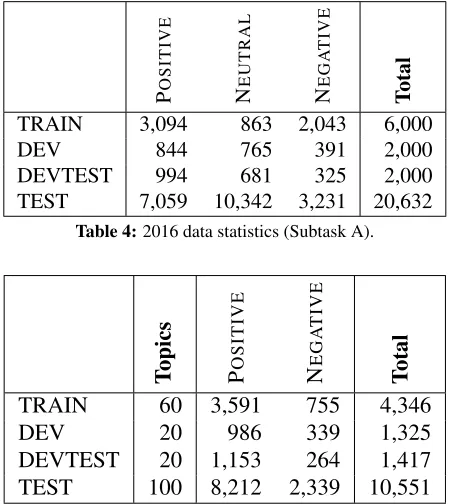
The consolidated statistics from the five annota-tors on a three-point scale for Subtask A are shown in Table 4. Note that, for consistency, we annotated the data for Subtask A on a five-point scale, which we then converted to a three-point scale.
Tweet Overall Sentiment Topic Sentiment Why would you still wear shorts when it’s this cold?! I
love how Britain see’s a bit of sun and they’re like ’OOOH LET’S STRIP!
POSITIVE Britain: NEGATIVE
Saturday without Leeds United is like Sunday dinner it doesn’t feel normal at all (Ryan)
NEGATIVE Leeds United: HIGHLYPOSITIVE
Who are you tomorrow? Will you make me smile or just bring me sorrow? #HottieOfTheWeek Demi Lovato
[image:5.612.77.538.58.159.2]NEUTRAL Demi Lovato: POSITIVE
Table 3:List of example tweets and annotations that were provided to the annotators.
P O S IT IV E N E U T R A L N E G A T IV E Total
TRAIN 3,094 863 2,043 6,000
DEV 844 765 391 2,000
DEVTEST 994 681 325 2,000
[image:5.612.73.298.191.443.2]TEST 7,059 10,342 3,231 20,632
Table 4:2016 data statistics (Subtask A).
Topics PO
S IT IV E N E G A T IV E Total
TRAIN 60 3,591 755 4,346
DEV 20 986 339 1,325
DEVTEST 20 1,153 264 1,417
TEST 100 8,212 2,339 10,551
Table 5:2016 data statistics (Subtasks B and D).
Topics HIG
H LY P O S IT IV E P O S IT IV E N E U T R A L N E G A T IV E H IG H LY N E G A T IV E Total
[image:5.612.74.299.472.580.2]TRAIN 60 437 3,154 1,654 668 87 6,000 DEV 20 53 933 675 296 43 2,000 DEVTEST 20 148 1,005 583 233 31 2,000 TEST 100 382 7,830 10,081 2,201 138 20,632
Table 6:2016 data statistics (Subtasks C and E).
As we use the same test tweets for all subtasks, the submission of results by participating teams was subdivided in two stages: (i) participants had to sub-mit results for Subtasks A, C, E, and (ii) only after the submission deadline for A, C, E had passed, we distributed to participants the unlabelled test data for Subtasks B and D.
Otherwise, since for Subtasks B and D we filter out the NEUTRALs, we would have leaked informa-tion about which the NEUTRALs are, and this infor-mation could have been used in Subtasks C and E.
Finally, as the same tweets can be selected for dif-ferent topics, we ended up with some duplicates; ar-guably, these are true duplicates for Subtask A only, as for the other subtasks the topics still differ. This includes 25 duplicates in TRAIN, 3 in DEV, 2 in DE-VTEST, and 116 in TEST. There is a larger number in TEST, as TEST is about twice as large as TRAIN, DEV, and DEVTEST combined. This is because we wanted a large TEST set with 100 topics and 200 tweets per topic on average for Subtasks C and E.
4 Evaluation Measures
This section discuss the evaluation measures for the five subtasks of our SemEval-2016 Task 4. A doc-ument describing the evaluation measures in detail6 (Nakov et al., 2016a), and a scoring software imple-menting all the five “official” measures, were made available to the participants via the task website to-gether with the training data.7
For Subtasks B to E, the datasets are each sub-divided into a number of “topics”, and the subtask needs to be carried out independently for each topic. As a result, each of the evaluation measures will be “macroaveraged” across the topics, i.e., we compute the measure individually for each topic, and we then average the results across the topics.
6http://alt.qcri.org/semeval2016/task4/ 7An earlier version of the scoring script contained a bug, to the effect that for Subtask B it was computingF1P N, and notρP N. This was detected only after the submissions were
closed, which means that participants to Subtask B who used the scoring system (and not their own implementation ofρP N) for
4.1 Subtask A: Message polarity classification
Subtask A is asingle-label multi-class(SLMC) clas-sification task. Each tweet must be classified as be-longing to exactly one of the following three classes C={POSITIVE, NEUTRAL, NEGATIVE}.
We adopt the same evaluation measure as the 2013-2015 editions of this subtask,F1P N:
F1P N = F
P 1 +F1N
2 (1)
FP
1 is theF1score for the POSITIVEclass:
F1P = 2π
PρP
πP +ρP (2)
Here,πP andρP denote precision and recall for the
POSITIVEclass, respectively:
πP = P P
P P +P U+P N (3)
ρP = P P
P P +U P +N P (4)
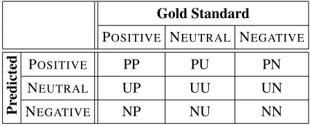
whereP P,U P,N P,P U,P N are the cells of the
confusion matrix shown in Table 7.
Gold Standard
POSITIVE NEUTRAL NEGATIVE
Pr
edicted
POSITIVE PP PU PN
NEUTRAL UP UU UN
[image:6.612.73.297.388.479.2]NEGATIVE NP NU NN
Table 7:The confusion matrix for Subtask A. CellXY stands for “the number of tweets that the classifier labeledXand the gold standard labells as Y”. P, U, N stand for POSITIVE,
NEUTRAL, NEGATIVE, respectively.
F1N is defined analogously, and the measure we
finally adopt isFP N
1 as from Equation 1.
4.2 Subtask B: Tweet classification according to a two-point scale
Subtask B is abinary classificationtask. Each tweet must be classified as either POSITIVEor NEGATIVE. For this subtask we adoptmacroaveraged recall:
ρP N = 1 2(ρ
P +ρN)
= 1
2(
P P P P +N P +
N N N N +P N)
(5)
In the above formula, ρP and ρN are the
posi-tive and the negaposi-tive class recall, respecposi-tively. Note thatU terms are entirely missing in Equation 5; this
is because we do not have the NEUTRALclass for SemEval-2016 Task 4, subtask A.
ρP N ranges in [0,1], where a value of 1 is
achieved only by the perfect classifier (i.e., the clas-sifier that correctly classifies all items), a value of 0 is achieved only by the perverse classifier (the clas-sifier that misclassifies all items), while0.5 is both
(i) the value obtained by a trivial classifier (i.e., the classifier that assigns all tweets to the same class – be it POSITIVEor NEGATIVE), and (ii) the expected value of a random classifier. The advantage ofρP N
over “standard” accuracy is that it is more robust to class imbalance. The accuracy of the majority-class classifier is the relative frequency (aka “prevalence”) of the majority class, that may be much higher than 0.5 if the test set is imbalanced. StandardF1is also
sensitive to class imbalance for the same reason. An-other advantage ofρP NoverF1is thatρP Nis
invari-ant with respect to switching POSITIVEwith NEG -ATIVE, whileF1 is not. See (Sebastiani, 2015) for
more details onρP N.
As we noted before, the training dataset, the de-velopment dataset, and the test dataset are each sub-divided into a number of topics, and Subtask B needs to be carried out independently for each topic. As a result, the evaluation measures discussed in this sec-tion are computed individually for each topic, and the results are then averaged across topics to yield the final score.
4.3 Subtask C: Tweet classification according to a five-point scale
Subtask C is an ordinal classification (OC – also known as ordinal regression) task, in which each tweet must be classified into exactly one of the classes in C={HIGHLYPOSITIVE, POS -ITIVE, NEUTRAL, NEGATIVE, HIGHLYNEGA -TIVE}, represented in our dataset by numbers in {+2,+1,0,−1,−2}, with a total order defined onC.
As our evaluation measure, we use macroaver-aged mean absolute error(M AEM):
M AEM(h, T e) = 1
|C|
|C|
X
j=1
1
|T ej| X
xi∈T ej
|h(xi)−yi|
where yi denotes the true label of item xi, h(xi)
is its predicted label, T ej denotes the set of test
documents whose true class is cj, |h(xi)−yi|
de-notes the “distance” between classes h(xi) and yi
(e.g., the distance between HIGHLYPOSITIVE and NEGATIVE is 3), and the “M” superscript indicates “macroaveraging”.
The advantage ofM AEM over “standard” mean
absolute error, which is defined as:
M AEµ(h, T e) = 1
|T e|
X
xi∈T e
|h(xi)−yi| (6)
is that it is robust to class imbalance (which is use-ful, given the imbalanced nature of our dataset). On perfectly balanced datasetsM AEM andM AEµare
equivalent.
Unlike the measures discussed in Sections 4.1 and 4.2,M AEM is a measure of error, and not accuracy,
and thus lower values are better. See (Baccianella et al., 2009) for more detail onM AEM.
Similarly to Subtask B, Subtask C needs to be car-ried out independently for each topic. As a result,
M AEM is computed individually for each topic,
and the results are then averaged across all topics to yield the final score.
4.4 Subtask D: Tweet quantification according to a two-point scale
Subtask D also assumes a binary quantification setup, in which each tweet is classified as POSITIVE or NEGATIVE. The task is to compute an estimate
ˆ
p(cj) of the relative frequency (in the test set) of
each of the classes.
The difference between binary classification (as from Section 4.2) and binary quantification is that errors of different polarity (e.g., a false positive and a false negative for the same class) can compensate each other in the latter. Quantification is thus a more lenient task since a perfect classifier is also a perfect quantifier, but a perfect quantifier is not necessarily a perfect classifier.
We adoptnormalized cross-entropy, better known as Kullback-Leibler Divergence (KLD). KLD was proposed as a quantification measure in (Forman, 2005), and is defined as follows:
KLD(ˆp, p,C) = X
cj∈C
p(cj) loge
p(cj)
ˆ
p(cj) (7)
KLDis a measure of the error made in estimating
a true distributionpover a setCof classes by means of a predicted distributionpˆ. LikeM AEM in
Sec-tion 4.3,KLD is a measure of error, which means
that lower values are better.KLDranges between 0
(best) and+∞(worst).
Note that the upper bound of KLDis not finite
since Equation 7 has predicted prevalences, and not true prevalences, at the denominator: that is, by making a predicted prevalencepˆ(cj)infinitely small
we can make KLD infinitely large. To solve this
problem, in computingKLDwe smooth bothp(cj)
andpˆ(cj)via additive smoothing, i.e.,
ps(cj) =
p(cj) +
(X
cj∈C
p(cj)) +· |C|
=p(cj) + 1 +· |C|
(8)
whereps(cj)denotes the smoothed version ofp(cj)
and the denominator is just a normalizer (same for the pˆs(cj)’s); the quantity = 2·|1T e| is used as a
smoothing factor, whereT edenotes the test set.
The smoothed versions of p(cj) and pˆ(cj) are
used in place of their original versions in Equation 7; as a result,KLDis always defined and still returns
a value of 0 whenpandpˆcoincide.
KLD is computed individually for each topic,
and the results are averaged to yield the final score.
4.5 Subtask E: Tweet quantification according to a five-point scale
Subtask E is an ordinal quantification (OQ) task, in which (as in OC) each tweet belongs exactly to one of the classes inC={HIGHLYPOSITIVE, POSI -TIVE, NEUTRAL, NEGATIVE, HIGHLYNEGATIVE}, where there is a total order onC. As in binary quan-tification, the task is to compute an estimatepˆ(cj)of
the relative frequencyp(cj)in the test tweets of all
The measure we adopt for OQ is the Earth Mover’s Distance(Rubner et al., 2000) (also known as the Vaser˘ste˘ın metric (R¨uschendorf, 2001)), a measure well-known in the field of computer vision.
EM D is currently the only known measure for or-dinal quantification. It is defined for the general case in which a distanced(c0, c00)is defined for each
c0, c00∈ C. When there is a total order on the classes inCandd(ci, ci+1) = 1for alli∈ {1, ...,(C −1)}
(as in our application), the Earth Mover’s Distance is defined as
EM D(ˆp, p) =
|C|−X1
j=1
|
j X
i=1
ˆ
p(ci)− j X
i=1
p(ci)| (9)
and can be computed in|C|steps from the estimated and true class prevalences.
Like KLD in Section 4.4, EM D is a measure
of error, so lower values are better; EM D ranges between 0 (best) and|C| −1(worst). See (Esuli and
Sebastiani, 2010) for more details onEM D.
As before, EM D is computed individually for each topic, and the results are then averaged across all topics to yield the final score.
5 Participants and Results
A total of 43 teams (see Table 15 at the end of the paper) participated in SemEval-2016 Task 4, repre-senting 25 countries; the country with the highest participation was China (5 teams), followed by Italy, Spain, and USA (4 teams each). The subtask with the highest participation was Subtask A (34 teams), followed by Subtask B (19 teams), Subtask D (14 teams), Subtask C (11 teams), and Subtask E (10 teams).
It was not surprising that Subtask A proved to be the most popular – it was a rerun from previous years; conversely, none among Subtasks B to E had previously been offered in precisely the same form. Quantification-related subtasks (D and E) generated 24 participations altogether, while subtasks with an ordinal nature (C and E) attracted 21 participations. Only three teams participated in all five subtasks; conversely, no less than 23 teams took part in one subtask only (with a few exceptions, Subtask A). Many teams that participated in more than one sub-task used essentially the same system for all of them, with little tuning to the specifics of each subtask.
Few trends stand out among the participating sys-tems. In terms of the supervised learning methods used, there is a clear dominance of methods based on deep learning, including convolutional neural net-works and recurrent neural netnet-works (and, in par-ticular, long short-term memory networks); the soft-ware libraries for deep learning most frequently used by the participants are Theano and Keras. Con-versely, kernel machines seem to be less frequently used than in the past, and the use of learning meth-ods other than the ones mentioned above is scarce.
The use of distant supervision is ubiquitous; this is natural, since there is an abundance of freely avail-able tweets labelled according to sentiment (possi-bly with silver labels only, e.g., emoticons), and it is intuitive that their use as additional training data could be helpful. Another ubiquitous technique is the use of word embeddings, usually generated via either word2vec (Mikolov et al., 2013) or GloVe (Pennington et al., 2014); most authors seem to use general-purpose, pre-trained embeddings, while some authors also use customized word embed-dings, trained either on the Tweet 2016 dataset or on tweet datasets of some sort.
Nothing radically new seems to have emerged with respect to text preprocessing; as in previous editions of this task, participants use a mix of by now obvious techniques, such as negation scope de-tection, elongation normalization, detection of am-plifiers and diminishers, plus the usual extraction of word n-grams, character n-grams, and POS n
-grams. The use of sentiment lexicons (alone or in combination with each other; general-purpose or Twitter-specific) is obviously still frequent.
In the next five subsections, we discuss the re-sults of the participating systems in the five sub-tasks, focusing on the techniques and tools that the top-ranked participants have used. We also focus on how the participants tailored (if at all) their approach to the specific subtask. When discussing a specific subtask, we will adopt the convention of adding to a team name a subscript which indicates the posi-tion in the ranking for that subtask that the team ob-tained; e.g., when discussing Subtask E, “Finki2”
5.1 Subtask A: Message polarity classification
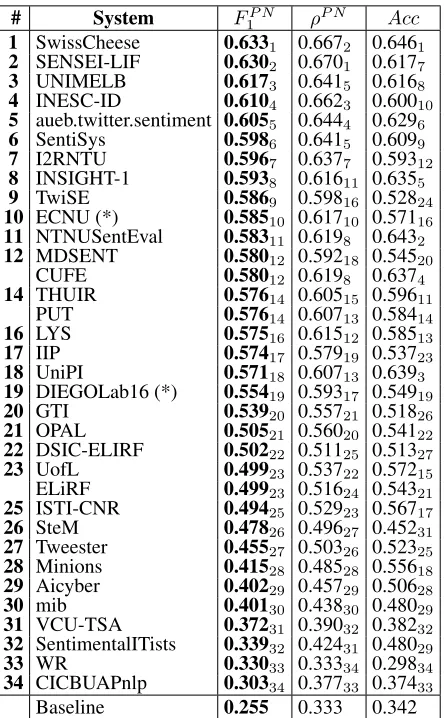
Table 8 ranks the systems submitted by the 34 teams who participated in Subtask A “Message Polarity Classification” in terms of the official measureFP N
1 .
We further show the result for two other measures,
ρP N (the measure that we adopted for Subtask B)
and accuracy (Acc = T P+T N+F PT P+T N+F N). We also
report the result for a baseline classifier that assigns to each tweet the POSITIVE class. For Subtask A evaluated using FP N
1 , this is the equivalent of the
majority class classifier for (binary or SLMC) clas-sification evaluated via vanilla accuracy, i.e., this is the “smartest” among the trivial policies that attempt to maximizeF1P N.
# System FP N
1 ρP N Acc
1 SwissCheese 0.6331 0.6672 0.6461
2 SENSEI-LIF 0.6302 0.6701 0.6177
3 UNIMELB 0.6173 0.6415 0.6168
4 INESC-ID 0.6104 0.6623 0.60010
5 aueb.twitter.sentiment 0.6055 0.6444 0.6296
6 SentiSys 0.5986 0.6415 0.6099
7 I2RNTU 0.5967 0.6377 0.59312
8 INSIGHT-1 0.5938 0.61611 0.6355
9 TwiSE 0.5869 0.59816 0.52824
10 ECNU (*) 0.58510 0.61710 0.57116
11 NTNUSentEval 0.58311 0.6198 0.6432
12 MDSENT 0.58012 0.59218 0.54520
CUFE 0.58012 0.6198 0.6374
14 THUIR 0.57614 0.60515 0.59611
PUT 0.57614 0.60713 0.58414
16 LYS 0.57516 0.61512 0.58513
17 IIP 0.57417 0.57919 0.53723
18 UniPI 0.57118 0.60713 0.6393
19 DIEGOLab16 (*) 0.55419 0.59317 0.54919
20 GTI 0.53920 0.55721 0.51826
21 OPAL 0.50521 0.56020 0.54122
22 DSIC-ELIRF 0.50222 0.51125 0.51327
23 UofL 0.49923 0.53722 0.57215
ELiRF 0.49923 0.51624 0.54321
25 ISTI-CNR 0.49425 0.52923 0.56717
26 SteM 0.47826 0.49627 0.45231
27 Tweester 0.45527 0.50326 0.52325
28 Minions 0.41528 0.48528 0.55618
29 Aicyber 0.40229 0.45729 0.50628
30 mib 0.40130 0.43830 0.48029
31 VCU-TSA 0.37231 0.39032 0.38232
32 SentimentalITists 0.33932 0.42431 0.48029
33 WR 0.33033 0.33334 0.29834
34 CICBUAPnlp 0.30334 0.37733 0.37433
Baseline 0.255 0.333 0.342
Table 8: Results for Subtask A “Message Polarity Classifica-tion” on the Tweet 2016 dataset. The systems are ordered by theirFP N
1 score. In each column the rankings according to the corresponding measure are indicated with a subscript. Teams marked as “(*)” are late submitters, i.e., their original submis-sion was deemed irregular by the organizers, and a revised sub-mission was entered after the deadline.
All 34 participating systems were able to outper-form the baseline on all three measures, with the ex-ception of one system that scored below the base-line onAcc. The top-scoring team (SwissCheese1)
used an ensemble of convolutional neural networks, differing in their choice of filter shapes, pooling shapes and usage of hidden layers. Word embed-dings generated via word2vec were also used, and the neural networks were trained by using distant supervision. Out of the 10 top-ranked teams, 5 teams (SwissCheese1, SENSEI-LIF2, UNIMELB3,
INESC-ID4, INSIGHT-18) used deep NNs of some
sort, and 7 teams (SwissCheese1, SENSEI-LIF2,
UNIMELB3, INESC-ID4, aueb.twitter.sentiment5,
I2RNTU7, INSIGHT-18) used either
general-purpose or task-specific word embeddings, gener-ated via word2vec or GloVe.
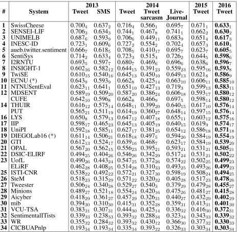
Historical results. We also tested the participat-ing systems on the test sets from the three previ-ous editions of this subtask. Participants were not allowed to use these test sets for training. Re-sults (measured on FP N
1 ) are reported in Table 9.
The top-performing systems on Tweet 2016 are also top-ranked on the test datasets from previous years. There is a general pattern: the top-ranked system in year x outperforms the top-ranked system in year
(x−1)on the official dataset of year(x−1).
Top-ranked systems tend to use approaches that are uni-versally strong, even when tested on out-of-domain test sets such as SMS, LiveJournal, or sarcastic tweets (yet, for sarcastic tweets, there are larger dif-ferences in rank compared to systems rankings on Tweet 2016). It is unclear where improvements come from: (a) the additional training data that we made available this year (in addition to Tweet-train-2013, which was used in 2013–2015), thus ef-fectively doubling the amount of training data, or (b) because of advancement of learning methods.
2013
2014
2015
2016
#
System
Tweet
SMS
Tweet
Tweet
Live-
Tweet Tweet
sarcasm Journal
1
SwissCheese
0.700
40.637
20.716
40.566
10.695
70.671
10.633
12
SENSEI-LIF
0.706
30.634
30.744
10.467
80.741
10.662
20.630
23
UNIMELB
0.687
60.593
90.706
60.449
110.683
90.651
40.617
34
INESC-ID
0.723
10.609
60.727
20.554
20.702
40.657
30.610
45
aueb.twitter.sentiment 0.666
70.618
50.708
50.410
170.695
70.623
70.605
56
SentiSys
0.714
20.633
40.723
30.515
40.726
20.644
50.598
67
I2RNTU
0.693
50.597
70.680
70.469
60.696
60.638
60.596
78
INSIGHT-1
0.602
160.582
120.644
150.391
230.559
230.595
160.593
89
TwiSE
0.610
150.540
160.645
130.450
100.649
130.621
80.586
910
ECNU (*)
0.643
90.593
90.662
80.425
140.663
100.606
110.585
1011
NTNUSentEval
0.623
110.641
10.651
100.427
130.719
30.599
130.583
1112
MDSENT
0.589
190.509
200.587
200.386
240.606
180.593
170.580
12CUFE
0.642
100.596
80.662
80.466
90.697
50.598
140.580
1214
THUIR
0.616
120.575
140.648
110.399
200.640
150.617
100.576
14PUT
0.565
210.511
190.614
190.360
270.648
140.597
150.576
1416
LYS
0.650
80.579
130.647
120.407
180.655
110.603
120.575
1617
IIP
0.598
170.465
230.645
130.405
190.640
150.619
90.574
1718
UniPI
0.592
180.585
110.627
170.381
250.654
120.586
180.571
1819
DIEGOLab16 (*)
0.611
140.506
210.618
180.497
50.594
200.584
190.554
1920
GTI
0.612
130.524
170.639
160.468
70.623
170.584
190.539
2021
OPAL
0.567
200.562
150.556
230.395
210.593
210.531
210.505
2122
DSIC-ELIRF
0.494
250.404
260.546
260.342
290.517
240.531
210.502
2223
UofL
0.490
260.443
240.547
250.372
260.574
220.502
250.499
23ELiRF
0.462
280.408
250.514
280.310
330.493
250.493
260.499
2325
ISTI-CNR
0.538
220.492
220.572
210.327
300.598
190.508
240.494
2526
SteM
0.518
230.315
290.571
220.320
320.405
280.517
230.478
2627
Tweester
0.506
240.340
280.529
270.540
30.379
290.479
280.455
2728
Minions
0.489
270.521
180.554
240.420
160.475
260.481
270.415
2829
Aicyber
0.418
290.361
270.457
290.326
310.440
270.432
290.402
2930
mib
0.394
300.310
300.415
310.352
280.359
310.413
310.401
3031
VCU-TSA
0.383
310.307
310.444
300.425
140.336
320.416
300.372
3132
SentimentalITists
0.339
330.238
330.393
320.288
340.323
340.343
330.339
3233
WR
0.355
320.284
320.393
320.430
120.366
300.377
320.330
33 [image:10.612.78.541.58.513.2]34
CICBUAPnlp
0.193
340.193
340.335
340.393
220.326
330.303
340.303
34 Table 9:Historical results for Subtask A “Message Polarity Classification”. The systems are ordered by their score on the Tweet 2016 dataset; the rankings on the individual datasets are indicated with a subscript. The meaning of “(*)” is as in Table 8.5.2 Subtask B: Tweet classification according to a two-point scale
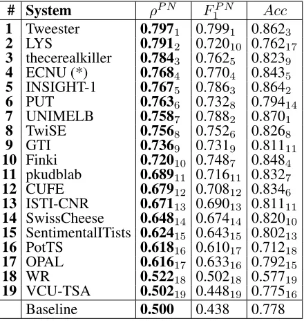
Table 11 ranks the 19 teams who participated in Subtask B “Tweet classification according to a two-point scale” in terms of the official measure ρP N.
Two other measures are reported, F1P N (the
mea-sure adopted for Subtask A) and accuracy (Acc). We also report the result of a baseline that assigns to each tweet the positive class. This is the “smartest” among the trivial policies that attempt to maximize
ρP N. This baseline always returnsρP N = 0.500.
Note however that this is also (i) the value re-turned by the classifier that assigns to each tweet the negative class, and (ii) the expected value returned by the random classifier; for more details see (Se-bastiani, 2015, Section 5), whereρP N is calledK.
The top-scoring team (Tweester1) used a
2013 2014 2015 2016 Year Tweet SMS Tweet Tweet Live- Tweet Tweet
sarcasm Journal
Best in 2016 0.723 0.641 0.744 0.566 0.741 0.671 0.633 Best in 2015 0.728 0.685 0.744 0.591 0.753 0.648 – Best in 2014 0.721 0.703 0.710 0.582 0.748 – –
[image:11.612.162.451.58.150.2]Best in 2013 0.690 0.685 – – – – –
Table 10:Historical results for the best systems for Subtask A “Message Polarity Classification” over the years 2013–2016.
# System ρP N FP N
1 Acc
1 Tweester 0.7971 0.7991 0.8623
2 LYS 0.7912 0.72010 0.76217
3 thecerealkiller 0.7843 0.7625 0.8239
4 ECNU (*) 0.7684 0.7704 0.8435
5 INSIGHT-1 0.7675 0.7863 0.8642
6 PUT 0.7636 0.7328 0.79414
7 UNIMELB 0.7587 0.7882 0.8701
8 TwiSE 0.7568 0.7526 0.8268
9 GTI 0.7369 0.7319 0.81111
10 Finki 0.72010 0.7487 0.8484
11 pkudblab 0.68911 0.71611 0.8327
12 CUFE 0.67912 0.70812 0.8346
13 ISTI-CNR 0.67113 0.69013 0.81111
14 SwissCheese 0.64814 0.67414 0.82010
15 SentimentalITists 0.62415 0.64315 0.80213
16 PotTS 0.61816 0.61017 0.71218
17 OPAL 0.61617 0.63316 0.79215
18 WR 0.52218 0.50218 0.57719
19 VCU-TSA 0.50219 0.44819 0.77516
[image:11.612.77.297.184.416.2]Baseline 0.500 0.438 0.778
Table 11:Results for Subtask B “Tweet classification according to a two-point scale” on the Tweet 2016 dataset. The systems are ordered by theirρP Nscore (higher is better). The meaning
of “(*)” is as in Table 8.
Out of the 10 top-ranked participating teams, 5 teams (Tweester1, LYS2,
INSIGHT-15, UNIMELB7, Finki10) used convolutional neural
networks; 3 teams (thecerealkiller3, UNIMELB7,
Finki10) submitted systems using recurrent
neu-ral networks; and 7 teams (Tweester1, LYS2,
INSIGHT-15, UNIMELB7, Finki10) incorporated in
their participating systems either general-purpose or task-specific word embeddings (generated via toolkits such as GloVe or word2vec).
Conversely, the use of classifiers such as support vector machines, which were dominant until a few years ago, seems to have decreased, with only one team (TwiSE8) in the top 10 using them.
[image:11.612.316.538.377.551.2]5.3 Subtask C: Tweet classification according to a five-point scale
Table 12 ranks the 11 teams who participated in Sub-task C “Tweet classification according to a five-point scale” in terms of the official measureM AEM; we
also showM AEµ(see Equation 6). We also report
the result of a baseline system that assigns to each tweet the middle class (i.e., NEUTRAL); for ordi-nal classification evaluated viaM AEM, this is the
majority-class classifier for (binary or SLMC) clas-sification evaluated via vanilla accuracy, i.e., this is (Baccianella et al., 2009) the “smartest” among the trivial policies that attempt to maximizeM AEM.
# System
M AE
MM AE
µ1
TwiSE
0.719
10.632
52
ECNU (*)
0.806
20.726
83
PUT
0.860
30.773
94
LYS
0.864
40.694
75
Finki
0.869
50.672
66
INSIGHT-1
1.006
60.607
37
ISTI-CNR
1.074
70.580
18
YZU-NLP
1.111
80.588
29
SentimentalITists
1.148
90.625
410
PotTS
1.237
100.860
1011
pkudblab
1.697
111.300
11Baseline
1.200
0.537
Table 12:Results for Subtask C “Tweet classification accord-ing to a five-point scale” on the Tweet 2016 dataset. The sys-tems are ordered by theirM AEM score (lower is better). The
meaning of “(*)” is as in Table 8.
The top-scoring team (TwiSE1) used a
# System KLD AE RAE
1 Finki 0.0341 0.0741 0.7073
2 LYS 0.0532 0.0994 0.8445
TwiSE 0.0532 0.1015 0.8646 4 INSIGHT-1 0.0544 0.0852 0.4231
5 GTI 0.0555 0.1046 1.20010
QCRI 0.0555 0.0953 0.8646
7 NRU-HSE 0.0847 0.1208 0.7674 8 PotTS 0.0948 0.15012 1.83812 9 pkudblab 0.0999 0.1097 0.9478 10 ECNU (*) 0.12110 0.14811 1.1719 11 ISTI-CNR 0.12711 0.1479 1.37111 12 SwissCheese 0.19112 0.1479 0.6382 13 UDLAP 0.26113 0.27413 2.97313 14 HSENN 0.39914 0.33614 3.93014
Baseline1 0.175 0.184 2.110
[image:12.612.76.298.60.265.2]Baseline2 0.887 0.242 1.155 Table 13:Results for Subtask D “Tweet quantification accord-ing to a two-point scale” on the Tweet 2016 dataset. The sys-tems are ordered by theirKLD score (lower is better). The
meaning of “(*)” is as in Table 8.
Only 2 of the 11 participating teams tuned their systems to exploit the ordinal (as opposed to binary, or single-label multi-class) nature of this subtask. The two teams who did exploit the ordinal nature of the problem are PUT3, which uses an ensemble
of ordinal regression approaches, and ISTI-CNR7,
which uses a tree-based approach to ordinal regres-sion. All other teams used general-purpose ap-proaches for single-label multi-class classification, in many cases relying (as for Subtask B) on convo-lutional neural networks, recurrent neural networks, and word embeddings.
5.4 Subtask D: Tweet quantification according to a two-point scale
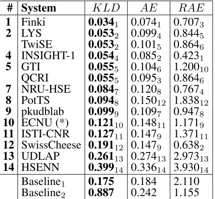
Table 13 ranks the 14 teams who participated in Sub-task D “Tweet quantification according to a two-point scale” on the official measure KLD. Two other measures are reported,absolute error(AE):
AE(p,p,ˆ C) = 1
|C|
X
c∈C
|pˆ(c)−p(c)| (10)
andrelative absolute error(RAE):
RAE(p,p,ˆ C) = 1
|C|
X
c∈C
|pˆ(c)−p(c)|
p(c) (11)
where the notation is the same as in Equation 7.
We also report the result of a “maximum like-lihood” baseline system (dubbed Baseline1). This
system assigns to each test topic the distribution of the training tweets (the union of TRAIN, DEV, DE-VTEST) across the classes. This is the “smartest” among the trivial policies that attempt to maximize
KLD. We also report the result of a further (less
smart) baseline system (dubbed Baseline2), i.e., one
that assigns a prevalence of 1 to the majority class (which happens to be the POSITIVE class) and a prevalence of 0 to the other class.
The top-scoring team (Finki1) adopts an approach
based on “classify and count”, a classification-oriented (instead of quantification-classification-oriented) ap-proach, using recurrent and convolutional neural networks, and GloVe word embeddings.
Indeed, only 5 of the 14 participating teams tuned their systems to the fact that it deals with quantifi-cation (as opposed to classifiquantifi-cation). Among the teams who do rely on quantification-oriented ap-proaches, teams LYS2 and HSENN14 used an
ex-isting structured prediction method that directly op-timizes KLD; teams QCRI5 and ISTI-CNR11 use
existing probabilistic quantification methods; team NRU-HSE7 uses an existing iterative quantification
method based on cost-sensitive learning. Interest-ingly, team TwiSE2 uses a “classify and count”
approach after comparing it with a quantification-oriented method (similar to the one used by teams LYS2 and HSENN14) on the development set, and
concluding that the former works better than the lat-ter. All other teams used “classify and count” ap-proaches, mostly based on convolutional neural net-works and word embeddings.
5.5 Subtask E: Tweet quantification according to a five-point scale
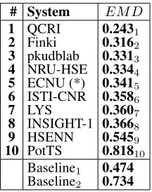
Table 14 lists the results obtained by the 10 partici-pating teams on Subtask E “Tweet quantification ac-cording to a five-point scale”. We also report the result of a “maximum likelihood” baseline system (dubbed Baseline1), i.e., one that assigns to each test
topic the same distribution, namely the distribution of the training tweets (the union of TRAIN, DEV, DEVTEST) across the classes; this is the “smartest” among the trivial policies (i.e., those that do not re-quire any genuine work) that attempt to maximize
We further report the result of less smart base-line system (dubbed Basebase-line2) – one that assigns
a prevalence of 1 to the majority class (which coin-cides with the POSITIVEclass) and a prevalence of 0 to all other classes.
# System EM D
1 QCRI 0.2431 2 Finki 0.3162 3 pkudblab 0.3313 4 NRU-HSE 0.3344 5 ECNU (*) 0.3415 6 ISTI-CNR 0.3586 7 LYS 0.3607 8 INSIGHT-1 0.3668 9 HSENN 0.5459 10 PotTS 0.81810
[image:13.612.132.240.144.281.2]Baseline1 0.474 Baseline2 0.734
Table 14:Results for Subtask E “Tweet quantification accord-ing to a five-point scale” on the Tweet 2016 dataset. The sys-tems are ordered by theirEM D score (lower is better). The meaning of “(*)” is as in Table 8.
Only 3 of the 10 participants tuned their systems to the specific characteristics of this subtask, i.e., to the fact that it deals with quantification (as opposed to classification)andto the fact that it has an ordinal (as opposed to binary) nature.
In particular, the top-scoring team (QCRI1) used
a novel algorithm explicitly designed for ordinal quantification, that leverages an ordinal hierarchy of binary probabilistic quantifiers.
Team NRU-HSE4 uses an existing
quantifica-tion approach based on cost-sensitive learning, and adapted it to the ordinal case.
Team ISTI-CNR6instead used a novel adaptation
to quantification of a tree-based approach to ordinal regression.
Teams LYS7 and HSENN9 also used an existing
quantification approach, but did not exploit the ordi-nal nature of the problem.
The other teams mostly used approaches based on “classify and count” (see Section 5.4), and viewed the problem as single-label multi-class (instead of ordinal) classification; some of these teams (notably, team Finki2) obtained very good results, which
tes-tifies to the quality of the (general-purpose) features and learning algorithm they used.
6 Conclusion and Future Work
We described SemEval-2016 Task 4 “Sentiment Analysis in Twitter”, which included five subtasks including three that represent a significant departure from previous editions. The three new subtasks fo-cused, individually or in combination, on two vari-ants of the basic “sentiment classification in Twitter” task that had not been previously explored within SemEval. The first variant adopts a five-point scale, which confers anordinalcharacter to the classifica-tion task. The second variant focuses on the correct estimation of the prevalence of each class of interest, a task which has been called quantification in the supervised learning literature. In contrast, previous years’ subtasks have focused on the correct labeling of individual tweets. As in previous years (2013– 2015), the 2016 task was very popular and attracted a total of 43 teams.
A general trend that emerges from SemEval-2016 Task 4 is that most teams who were ranked at the top in the various subtasks used deep learning, includ-ing convolutional NNs, recurrent NNs, and (general-purpose or task-specific) word embeddings. In many cases, the use of these techniques allowed the teams using them to obtain good scores even without tun-ing their system to the specifics of the subtask at hand, e.g., even without exploiting the ordinal na-ture of the subtask – for Subtasks C and E – or the quantification-related nature of the subtask – for Subtasks D and E. Conversely, several teams that have indeed tuned their system to the specifics of the subtask at hand, but have not used deep learning techniques, have performed less satisfactorily. This is a further confirmation of the power of deep learn-ing techniques for tweet sentiment analysis.
Concerning Subtasks D and E, if quantification-based subtasks are proposed again, we think it might be a good idea to generate, for each test topic ti,
multiple “artificial” test topicst1i, t2i, ..., where class
prevalences are altered with respect to the ones ofti
by means of selectively removing fromtitweets
By varying the amount of removed tweets at will, one may obtain many test topics, thus augmenting the magnitude of the experimentation at will while at the same time keeping constant the amount of man-ual annotation needed.
In terms of possible follow-ups of this task, it might be interesting to have a subtask whose goal is to distinguish tweets that are NEUTRAL about the topic (i.e., do not express any opinion about the topic) from tweets that express a FAIR opin-ion (i.e., lukewarm, intermediate between POSITIVE and NEGATIVE) about the topic.
Another possibility is to have a multi-lingual tweet sentiment classification subtask, where train-ing examples are provided for the same topic for two languages (e.g., English and Arabic), and where par-ticipants can improve their performance on one lan-guage by leveraging the training examples for the other language via transfer learning. Alternatively, it might be interesting to include a cross-lingual tweet sentiment classification subtask, where training ex-amples are provided for a given language (e.g., En-glish) but not for the other (e.g., Arabic); the second language could be also a surprise language, which could be announced at the last moment.
References
Omar Abdelwahab and Adel Elmaghraby. 2016. UofL at SemEval-2016 Task 4: Multi domain word2vec for Twitter sentiment classification. InProceedings of the 10th International Workshop on Semantic Evaluation (SemEval 2016), San Diego, US.
Ram´on Astudillo and Silvio Amir. 2016. INESC-ID at SemEval-2016 Task 4: Reducing the problem of out-of-embedding words. InProceedings of the 10th Inter-national Workshop on Semantic Evaluation (SemEval 2016), San Diego, US.
Giuseppe Attardi and Daniele Sartiano. 2016. UniPI at SemEval-2016 Task 4: Convolutional neural networks for sentiment classification. InProceedings of the 10th International Workshop on Semantic Evaluation (Se-mEval 2016), San Diego, US.
Stefano Baccianella, Andrea Esuli, and Fabrizio Sebas-tiani. 2009. Evaluation measures for ordinal regres-sion. In Proceedings of the 9th IEEE International Conference on Intelligent Systems Design and Appli-cations (ISDA 2009), pages 283–287, Pisa, IT. Stefano Baccianella, Andrea Esuli, and Fabrizio
Sebas-tiani. 2010. SentiWordNet 3.0: An enhanced lexical
resource for sentiment analysis and opinion mining. In Proceedings of the 7th Conference on Language Re-sources and Evaluation (LREC 2010), Valletta, MT. Alexandra Balahur. 2016. OPAL at SemEval-2016 Task
4: the Challenge of Porting a Sentiment Analysis Sys-tem to the ”Real” World. InProceedings of the 10th International Workshop on Semantic Evaluation (Se-mEval 2016), San Diego, US.
Georgios Balikas and Massih-Reza Amini. 2016. TwiSE at SemEval-2016 Task 4: Twitter sentiment classifica-tion. InProceedings of the 10th International Work-shop on Semantic Evaluation (SemEval 2016), San Diego, US.
Johan Bollen, Huina Mao, and Xiao-Jun Zeng. 2011. Twitter mood predicts the stock market. Journal of Computational Science, 2(1):1–8.
Javier Borge-Holthoefer, Walid Magdy, Kareem Dar-wish, and Ingmar Weber. 2015. Content and net-work dynamics behind Egyptian political polarization on Twitter. InProceedings of the 18th ACM Confer-ence on Computer Supported Cooperative Work and Social Computing (CSCW 2015), pages 700–711, Van-couver, CA.
Gerard Briones and Kasun Amarasinghe. 2016. VCU-TSA at SemEval-2016 Task 4: Sentiment analysis in Twitter. InProceedings of the 10th International Workshop on Semantic Evaluation (SemEval 2016), San Diego, US.
S. Burton and A. Soboleva. 2011. Interactive or reac-tive? Marketing with Twitter. Journal of Consumer Marketing, 28(7):491–499.
Esteban Castillo, Ofelia Cervantes, Darnes Vilari˜no, and David B´aez. 2016. UDLAP at SemEval-2016 Task 4: Sentiment quantification using a graph based rep-resentation. InProceedings of the 10th International Workshop on Semantic Evaluation (SemEval 2016), San Diego, US.
Calin-Cristian Ciubotariu, Marius-Valentin Hrisca, Mi-hail Gliga, Diana Darabana, Diana Trandabat, and Adrian Iftene. 2016. Minions at SemEval-2016 Task 4: Or how to boost a student’s self esteem. In Proceed-ings of the 10th International Workshop on Semantic Evaluation (SemEval 2016), San Diego, US.
Vittoria Cozza and Marinella Petrocchi. 2016. mib at SemEval-2016 Task 4: Exploiting lexicon based fea-tures for sentiment analysis in Twitter. InProceedings of the 10th International Workshop on Semantic Eval-uation (SemEval 2016), San Diego, US.
Jan Deriu, Maurice Gonzenbach, Fatih Uzdilli, Aurelien Lucchi, Valeria De Luca, and Martin Jaggi. 2016. SwissCheese at SemEval-2016 Task 4: Sentiment classification using an ensemble of convolutional neu-ral networks with distant supervision. InProceedings of the 10th International Workshop on Semantic Eval-uation (SemEval 2016), San Diego, US.
Peter S. Dodds, Kameron D. Harris, Isabel M. Kloumann, Catherine A. Bliss, and Christopher M. Danforth. 2011. Temporal patterns of happiness and information in a global social network: Hedonometrics and Twitter. PLoS ONE, 6(12).
Steven Du and Xi Zhang. 2016. Aicyber at SemEval-2016 Task 4: i-vector based sentence representation. InProceedings of the 10th International Workshop on Semantic Evaluation (SemEval 2016), San Diego, US. Andrea Esuli and Fabrizio Sebastiani. 2010. Sentiment quantification. IEEE Intelligent Systems, 25(4):72–75. Andrea Esuli and Fabrizio Sebastiani. 2015. Opti-mizing text quantifiers for multivariate loss functions. ACM Transactions on Knowledge Discovery and Data, 9(4):Article 27.
Andrea Esuli. 2016. ISTI-CNR at SemEval-2016 Task 4: Quantification on an ordinal scale. InProceedings of the 10th International Workshop on Semantic Eval-uation (SemEval 2016), San Diego, US.
Cosmin Florean, Oana Bejenaru, Eduard Apostol, Oc-tavian Ciobanu, Adrian Iftene, and Diana Trandabat. 2016. SentimentalITists at SemEval-2016 Task 4: Building a Twitter sentiment analyzer in your back-yard. InProceedings of the 10th International Work-shop on Semantic Evaluation (SemEval 2016), San Diego, US.
George Forman. 2005. Counting positives accurately despite inaccurate classification. In Proceedings of the 16th European Conference on Machine Learning (ECML 2005), pages 564–575, Porto, PT.
George Forman. 2008. Quantifying counts and costs via classification. Data Mining and Knowledge Discov-ery, 17(2):164–206.
Jasper Friedrichs. 2016. IIP at SemEval-2016 Task 4: Prioritizing classes in ensemble classification for sen-timent analysis of tweets. InProceedings of the 10th International Workshop on Semantic Evaluation (Se-mEval 2016), San Diego, US.
Hang Gao and Tim Oates. 2016. MDSENT at SemEval-2016 Task 4: Supervised system for message polar-ity classification. In Proceedings of the 10th Inter-national Workshop on Semantic Evaluation (SemEval 2016), San Diego, US.
Stavros Giorgis, Apostolos Rousas, John Pavlopoulos, Prodromos Malakasiotis, and Ion Androutsopoulos. 2016. aueb.twitter.sentiment at SemEval-2016 Task
4: A weighted ensemble of SVMs for Twitter sen-timent analysis. In Proceedings of the 10th Inter-national Workshop on Semantic Evaluation (SemEval 2016), San Diego, US.
Helena Gomez, Darnes Vilari˜no, Grigori Sidorov, and David Pinto Avenda˜no. 2016. CICBUAPnlp at SemEval-2016 Task 4: Discovering Twitter polarity using enhanced embeddings. In Proceedings of the 10th International Workshop on Semantic Evaluation (SemEval 2016), San Diego, US.
Hussam Hamdan. 2016. SentiSys at SemEval-2016 Task 4: Feature-based system for sentiment analysis in Twitter. InProceedings of the 10th International Workshop on Semantic Evaluation (SemEval 2016), San Diego, US.
Yunchao He, Liang-Chih Yu, Chin-Sheng Yang, K. Robert Lai, and Weiyi Liu. 2016. YZU-NLP at SemEval-2016 Task 4: Ordinal sentiment classifica-tion using a recurrent convoluclassifica-tional network. In Pro-ceedings of the 10th International Workshop on Se-mantic Evaluation (SemEval 2016), San Diego, US. Brage Ekroll Jahren, Valerij Fredriksen, Bj¨orn Gamb¨ack,
and Lars Bungum. 2016. NTNUSentEval at SemEval-2016 Task 4: Combining general classifiers for fast Twitter sentiment analysis. InProceedings of the 10th International Workshop on Semantic Evaluation (Se-mEval 2016), San Diego, US.
Jonathan Juncal-Mart´ınez, Tamara ´Alvarez-L´opez, Milagros Fern´andez-Gavilanes, Enrique Costa-Montenegro, and Francisco Javier Gonz´alez-Casta˜no. 2016. GTI at SemEval-2016 Task 4: Training a naive Bayes classifier using features of an unsupervised system. In Proceedings of the 10th International Workshop on Semantic Evaluation (SemEval 2016), San Diego, US.
Nikolay Karpov, Alexander Porshnev, and Kirill Rudakov. 2016. NRU-HSE at SemEval-2016 Task 4: The open quantification library with two iterative methods. In Proceedings of the 10th International Workshop on Semantic Evaluation (SemEval 2016), San Diego, US.
Mesut Kaya, Guven Fidan, and Ismail Hakki Toroslu. 2013. Transfer learning using Twitter data for improv-ing sentiment classification of Turkish political news. In Proceedings of the 28th International Symposium on Computer and Information Sciences (ISCIS 2013), pages 139–148, Paris, FR.
Mateusz Lango, Dariusz Brzezinski, and Jerzy Ste-fanowski. 2016. PUT at SemEval-2016 Task 4: The ABC of Twitter sentiment analysis. InProceedings of the 10th International Workshop on Semantic Evalua-tion (SemEval 2016), San Diego, US.
supervi-sion: Political forecasting with Twitter. In Proceed-ings of the 13th Conference of the European Chap-ter of the Association for Computational Linguistics (EACL 2012), pages 603–612, Avignon, FR.
Eugenio Mart´ınez-C´amara, Maria Teresa Mart´ın-Valdivia, Luis Alfonso Ure˜na L´opez, and Arturo Mon-tejo R´aez. 2014. Sentiment analysis in Twitter. Natural Language Engineering, 20(1):1–28.
Yelena Mejova, Ingmar Weber, and Michael W. Macy, editors. 2015. Twitter: A Digital Socioscope. Cam-bridge University Press, CamCam-bridge, UK.
Tomas Mikolov, Wen-Tau Yih, and Geoffrey Zweig. 2013. Linguistic Regularities in Continuous Space Word Representations. In Proceedings of the 2013 Conference of the North American Chapter of the Association for Computational Linguistics (NAACL 2013), pages 746–751, Atlanta, US.
Victor Martinez Morant, Llu´ıs-F. Hurtado, and Ferran Pla. 2016. DSIC-ELIRF at SemEval-2016 Task 4: Message polarity classification in Twitter using a sup-port vector machine approach. InProceedings of the 10th International Workshop on Semantic Evaluation (SemEval 2016), San Diego, US.
Mahmoud Nabil, Amir Atyia, and Mohamed Aly. 2016. CUFE at SemEval-2016 Task 4: A gated recurrent model for sentiment classification. InProceedings of the 10th International Workshop on Semantic Evalua-tion (SemEval 2016), San Diego, US.
Preslav Nakov, Sara Rosenthal, Zornitsa Kozareva, Veselin Stoyanov, Alan Ritter, and Theresa Wilson. 2013. SemEval-2013 Task 2: Sentiment analysis in Twitter. InProceedings of the 7th International Work-shop on Semantic Evaluation (SemEval 2013), pages 312–320, Atlanta, US.
Preslav Nakov, Alan Ritter, Sara Rosenthal, Fab-rizio Sebastiani, and Veselin Stoyanov. 2016a. Evaluation measures for the SemEval-2016 Task 4 “Sentiment analysis in Twitter”. Available from http://alt.qcri.org/semeval2016/task4/.
Preslav Nakov, Sara Rosenthal, Svetlana Kiritchenko, Saif M. Mohammad, Zornitsa Kozareva, Alan Ritter, Veselin Stoyanov, and Xiaodan Zhu. 2016b. Devel-oping a successful SemEval task in sentiment analysis of Twitter and other social media texts. Language Re-sources and Evaluation, 50(1):35–65.
Brendan O’Connor, Ramnath Balasubramanyan, Bryan R. Routledge, and Noah A. Smith. 2010. From tweets to polls: Linking text sentiment to public opinion time series. InProceedings of the 4th AAAI Conference on Weblogs and Social Media (ICWSM 2010), Washington, US.
Elisavet Palogiannidi, Athanasia Kolovou, Fenia Christopoulou, Filippos Kokkinos, Elias Iosif, Niko-laos Malandrakis, Haris Papageorgiou, Shrikanth
Narayanan, and Alexandros Potamianos. 2016. Tweester at SemEval-2016 Task 4: Sentiment analysis in Twitter using semantic-affective model adaptation. InProceedings of the 10th International Workshop on Semantic Evaluation (SemEval 2016), San Diego, US. Jeffrey Pennington, Richard Socher, and Christopher D. Manning. 2014. GloVe: Global vectors for word representation. InProceedings of the Conference on Empirical Methods in Natural Language Processing (EMNLP 2014), pages 1532–1543, Doha, QA. Muhammad A. Qureshi, Colm O’Riordan, and Gabriella
Pasi. 2013. Clustering with error estimation for moni-toring reputation of companies on Twitter. In Proceed-ings of the 9th Asia Information Retrieval Societies Conference (AIRS 2013), pages 170–180, Singapore, SN.
Stefan R¨abiger, Mishal Kazmi, Y¨ucel Saygın, Peter Sch¨uller, and Myra Spiliopoulou. 2016. SteM at SemEval-2016 Task 4: Applying active learning to im-prove sentiment classification. InProceedings of the 10th International Workshop on Semantic Evaluation (SemEval 2016), San Diego, US.
Alan Ritter, Sam Clark, and Oren Etzioni. 2011. Named entity recognition in tweets: An experimental study. InProceedings of the Conference on Empirical Meth-ods in Natural Language Processing (EMNLP 2011), pages 1524–1534, Edinburgh, UK.
Sara Rosenthal, Alan Ritter, Preslav Nakov, and Veselin Stoyanov. 2014. SemEval-2014 Task 9: Sentiment analysis in Twitter. InProceedings of the 8th Inter-national Workshop on Semantic Evaluation (SemEval 2014), pages 73–80, Dublin, IE.
Sara Rosenthal, Preslav Nakov, Svetlana Kiritchenko, Saif Mohammad, Alan Ritter, and Veselin Stoyanov. 2015. SemEval-2015 Task 10: Sentiment analysis in Twitter. InProceedings of the 9th International Work-shop on Semantic Evaluation (SemEval 2015), pages 451–463, Denver, US.
Mickael Rouvier and Benoit Favre. 2016. SENSEI-LIF at SemEval-2016 Task 4: Polarity embedding fusion for robust sentiment analysis. InProceedings of the 10th International Workshop on Semantic Evaluation (SemEval 2016), San Diego, US.
Yossi Rubner, Carlo Tomasi, and Leonidas J. Guibas. 2000. The Earth Mover’s Distance as a metric for im-age retrieval. International Journal of Computer Vi-sion, 40(2):99–121.
Ludger R¨uschendorf. 2001. Wasserstein metric. In Michiel Hazewinkel, editor,Encyclopaedia of Mathe-matics. Kluwer Academic Publishers, Dordrecht, NL. Abeed Sarker. 2016. DIEGOLab16 at SemEval-2016
Task 4: Sentiment analysis in Twitter using centroids, clusters, and sentiment lexicons. InProceedings of the 10th International Workshop on Semantic Evaluation (SemEval 2016), San Diego, US.
Fabrizio Sebastiani. 2015. An axiomatically derived measure for the evaluation of classification algorithms. InProceedings of the 5th ACM International Confer-ence on the Theory of Information Retrieval (ICTIR 2015), pages 11–20, Northampton, US.
Uladzimir Sidarenka. 2016. PotTS at SemEval-2016 Task 4: Sentiment analysis of Twitter using character-level convolutional neural networks. In Proceedings of the 10th International Workshop on Semantic Eval-uation (SemEval 2016), San Diego, US.
Dario Stojanovski, Gjorgji Strezoski, Gjorgji Madjarov, and Ivica Dimitrovski. 2016. Finki at SemEval-2016 Task 4: Deep learning architecture for Twitter sen-timent analysis. In Proceedings of the 10th Inter-national Workshop on Semantic Evaluation (SemEval 2016), San Diego, US.
David Vilares, Yerai Doval, Miguel A. Alonso, and Car-los G´omez-Rodr´ıguez. 2016. LYS at SemEval-2016 Task 4: Exploiting neural activation values for Twit-ter sentiment classification and quantification. In Pro-ceedings of the 10th International Workshop on Se-mantic Evaluation (SemEval 2016), San Diego, US. Steven Xu, HuiZhi Liang, and Tim Baldwin. 2016.
UNIMELB at SemEval-2016 Task 4: An ensemble of neural networks and a word2vec based model for sen-timent classification. InProceedings of the 10th Inter-national Workshop on Semantic Evaluation (SemEval 2016), San Diego, US.
Vikrant Yadav. 2016. thecerealkiller at SemEval-2016 Task 4: Deep learning based system for classifying sentiment of tweets on two point scale. In Proceed-ings of the 10th International Workshop on Semantic Evaluation (SemEval 2016), San Diego, US.
Zhengchen Zhang, Chen Zhang, Dongyan Huang, Wu Fuxiang, Weisi Lin, and Minghui Dong. 2016. I2RNTU at SemEval-2016 Task 4: Classifier fusion for polarity classification in Twitter. InProceedings of the 10th International Workshop on Semantic Evalua-tion (SemEval 2016), San Diego, US.
Subtasks Team ID Affiliation Nation Paper
A Aicyber Aicyber.com Singapore; China (Du and Zhang, 2016) A aueb.twitter.sentiment Department of Informatics, Athens University of Economics and Business Greece (Giorgis et al., 2016)
A CICBUAPnlp Instituto Polit`ecnico Nacional Mexico (Gomez et al., 2016) Benem`erita Universidad Autonoma de Puebla
A B CUFE Cairo University Egypt (Nabil et al., 2016) A DIEGOLab16 Arizona State University USA (Sarker, 2016) A DSIC-ELIRF Universitat Polit`ecnica de Val`encia Spain (Morant et al., 2016) A B C D E ECNU East China Normal University China (Zhou et al., 2016) A ELiRF Universitat Polit`ecnica de Val`encia Spain
B C D E Finki Saints Cyril and Methodius University, Skopje Macedonia (Stojanovski et al., 2016) A B D GTI AtlantTIC Centre, University of Vigo Spain (Juncal-Mart´ınez et al., 2016)
D E HSENN National Research University Higher School of Economics Russia
A I2RNTU Institute for Infocomm Research, A*STAR Singapore (Zhang et al., 2016) School of Computer Engineering, Nanyang Technological University
A IIP Infosys Limited India (Friedrichs, 2016)
A INESC-ID INESC-ID, Lisboa Portugal (Astudillo and Amir, 2016) Instituto Superior T´ecnico, Universidade de Lisboa
A B C D E INSIGHT-1 INSIGHT Research Centre, National University of Ireland, Galway Ireland (Ruder et al., 2016) AYLIEN Inc.
A B C D E LYS Universidade da Coru˜na Spain (Vilares et al., 2016) Universidade de Vigo
A MDSENT University of Maryland Baltimore County USA (Gao and Oates, 2016) A mib Istituto di Informatica e Telematica, Consiglio Nazionale delle Ricerche Italy (Cozza and Petrocchi, 2016) A Minions University of Iasi Romania (Ciubotariu et al., 2016) A B C D E ISTI-CNR Istituto di Scienza e Tecnologie dell’Informazione, Consiglio Nazionale delle Ricerche Italy (Esuli, 2016)
D E NRU-HSE National Research University Higher School of Economics Russia (Karpov et al., 2016) A NTNUSentEval Norwegian University of Science and Technology Norway (Jahren et al., 2016) A B OPAL European Commission Joint Research Centre Italy (Balahur, 2016)
B C D E pkudblab Peking University China
B C D E PotTS University of Potsdam Germany (Sidarenka, 2016) Retresco GmbH
A B C PUT Poznan University of Technology Poland (Lango et al., 2016) D E QCRI (**) Qatar Computing Research Institute Qatar (Da San Martino et al., 2016) A SENSEI-LIF Aix-Marseille University - CNRS - LIF France (Rouvier and Favre, 2016) A B C SentimentalITists University of Iasi Romania (Florean et al., 2016) A SentiSys Aix-Marseille University France (Hamdan, 2016)
A SteM
Sabanci University
Turkey
(R¨abiger et al., 2016) Marmara University
Otto-von-Guericke University Magdeburg Germany
A B D SwissCheese ETH Z¨urich Switzerland (Deriu et al., 2016) B thecerealkiller Amazon.in India (Yadav, 2016)
A THUIR Tsinghua University China
A B Tweester
School of ECE, National Technical University of Athens
Greece (Palogiannidi et al., 2016) School of ECE, Technical University of Crete
Department of Informatics, University of Athens Signal Analysis and Interpretation Laboratory (SAIL) Institute for Language & Speech Processing - ILSP
A B C D TwiSE University of Grenoble-Alpes France (Balikas and Amini, 2016) D UDLAP Universidad de las Am´ericas Puebla (UDLAP) Mexico (Castillo et al., 2016) A B UNIMELB University of Melbourne Australia (Xu et al., 2016) A UniPI Universit`a di Pisa Italy (Attardi and Sartiano, 2016) A UofL University of Louisville USA (Abdelwahab and Elmaghraby, 2016) A B VCU-TSA Virginia Commonwealth University USA (Briones and Amarasinghe, 2016)
A B WR WR Hong Kong
C YZU-NLP Yuan Ze University, Taoyuan Taiwan (He et al., 2016) Yunnan University, Kunming China
[image:18.612.75.540.71.653.2]34 19 11 14 10 Total