Abstract— We consider the analytical modeling of a condition-based monitoring for a system which is subject to degradation over time. The system condition is described by a monotonically increasing stochastic process that can be observed at discrete times by means of imperfect inspections. In addition to the critical threshold, for each time point of inspection a replacement threshold is introduced. The decision rule when checking system suitability for use in the upcoming time interval is considered. The expressions for the probabilities of correct and incorrect decisions when checking system suitability are derived with considering the results of previous inspections. A specific deterioration process is used to illustrate the proposed general expressions for the probabilities of correct and incorrect decisions. To determine the optimal threshold at each time of inspection, it is proposed to use criteria such as the maximum a posteriori probability criterion, minimum Bayes risk criterion and minimum total error probability criterion. A numerical example illustrates the efficiency of the proposed approach.
Index Terms—Condition based maintenance, suitability checking, decision rule, optimal replacement threshold
I. INTRODUCTION
ONDITION-based maintenance (CBM) is a type of maintenance wherein maintenance decisions depend on the information obtained from the condition monitoring (CM). Obviously, CM is preferred among other maintenance techniques in cases where system deterioration can be measured and where the system enters the failed state when at least one state parameter deteriorates beyond the level of functional failure. Condition-based maintenance allows to assess the system state via continuous monitoring or inspections at discrete times. The growing interest about CM is evident from the large number of studies related to various mathematical models and optimization techniques. Most of the existing mathematical models of CM with inspections at discrete times can be classified into two groups: models of CM with perfect inspections and models of CM with imperfect inspections. The latter is the subject of this study.
Maintenance models with imperfect inspections usually consider two types of errors: “false positives” (false alarms) with probability α and “false negatives” (i.e. non-detecting of failure) with probability β; for example [1]. Such models
Manuscript received June 20, 2015; revised July 14, 2015.
A. Raza is with the Department of the President’s Affairs, Overseas Projects & Maintenance, Abu Dhabi, 000372, UAE (e-mail: [email protected]).
V. Ulansky is with the Electronics Department, National Aviation University, Kiev, 03058 Ukraine. (00380632754982; e-mail: [email protected])
are not CBM models because in reality the error probabilities are not constant coefficients but depend on time and the parameters of the deterioration process. Moreover, such models depend on the results of previous multiple inspections, as shown in [2, 3]. Therefore, we analyze only those studies in which the probabilistic indicators of the inspection errors depend on the deterioration process parameters. In [2], CBM policies with imperfect operability checks are analyzed. The probabilities of four possible correct and incorrect decisions when checking system operability are considered. The proposed expressions depend on the deterioration process parameters and the results of previous inspections. In [4], the result of a measurement includes the original deterioration process along with a normally distributed measurement error. Based on this model, a decision rule was analyzed and optimal monitoring policies were found. The same approach was used in [5] to include measurement error in a Wiener diffusion process-based degradation model. A similar approach was used in [6] to find the likelihood for more than one inspection. A simple extension to the Bayesian updating model was proposed, such that the model can incorporate the results of inaccurate measurements. In [7], the threshold-type policy introduced for the maintenance action. If the system deterioration stage is less than the minimal threshold, no maintenance is conducted; if the system deterioration stage is found to be between the minimal threshold and the major threshold, than minimal maintenance is carried out; and major maintenance is performed if the system deterioration stage is larger than the major maintenance threshold. The model is based on a stochastic Petri net. In [8], an optimal replacement policy is considered when the state of system is unknown but can be estimated based on the observed condition. A proportional hazards model is used to represent the system's degradation. The optimization of the optimal maintenance policy is formulated as a partially observed Markov decision process, and the problem is solved using dynamic programming. In [9], the analytical model is developed for condition-based imperfect inspections of a stochastically deteriorating single-unit system. The system condition is described by a stochastic process with monotonically decreasing realizations. The analytical expressions for the probabilities of correct and incorrect decisions are derived. However, the proposed model does not consider the results of previous inspections.
In this study, we consider a stochastically and continuously deteriorating system whose state is described by one parameter and monitored through imperfect inspections. The system state parameter is assumed to be a
Optimal Thresholds for Stochastically
Deteriorating Systems
A.
Raza and V. Ulansky
stochastic process with monotonically increasing realizations. When the system state parameter exceeds its functional failure level FF, the system passes into the failed state and corrective replacement is necessary. The system state is inspected at discrete instants of time. When checking the system state parameter, errors are possible due to the imperfection of the measuring equipment. Each system rejected by the results of inspection is replaced by a new one. Currently, when checking the operability of a one-parameter system the following decision rule is used: if z(tk)
< FF, the system is judged operable and allowed for intended use in the interval (tk, tk+1), k = 1, 2, … , otherwise
(i.e. when z(tk) ≥ FF) the system is judged inoperable and
beyond repair, where z(tk) is the measured value of the
system state parameter at time tk. When optimizing this
decision rule, different criteria such as, criterion of minimum Bayes risk, criterion of maximum a posteriori probability and criterion of minimum total error probability are used. Each of these criteria is expressed through the probabilities of a “false failure” α(tk) and an “undetected failure” β(tk),
which are computed for the time point tk by using equations
described in previous studies, for example, in [10]. Therefore, when optimizing the decision rule by using the probabilities α(tk) and β(tk) the behavior of the system state
parameter in the interval (tk, tk+1) is not considered. Indeed, if
the operable system was falsely rejected at time point tk, then
this decision would be correct if the system further failed in the interval (tk, tk+1). Analogically, the decision that the
operable system at time point tk was judged as operable
would be wrong if this system further failed in the interval (tk, tk+1). Thus, when determining the decision rule and
probabilities α(tk) and β(tk), considering the behavior of the
system state parameter in the coming interval of operation is necessary.
In this study, we propose a mathematical model for calculating the probabilities of correct and incorrect decisions while considering the behavior of the system in the interval between inspections and the results of previous inspections. The proposed approach allows determining the optimal threshold PFk (PFk< FF) at time of inspection tk (k
= 1, 2, …). This will obviously reduce the probability of a functional failure in the intervals between inspections and improve the economic efficiency of the maintenance policy.
II. THE SPACE OF EVENTS
Let the state of a system be determined by the values of one parameter X(t), which is a stochastic process with monotonically increasing realizations. A system is inspected at successive times tk (k = 1, 2, …) under an infinite horizon
planning, where t0 = 0. Denote the result of measuring the
parameter X(t) at time tk as
t
kX
t
kY
t
kZ
, (1)where Y(tk) is the measurement error of the system state
parameter at time tk. We assume further that X(tk) and Y(tk)
are independent random variables.
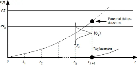
[image:2.595.308.546.52.165.2]A typical realization of the stochastic process X(t) measured at time tk is shown in Fig. 1.
Fig. 1. Realisation of the stochastic process X(t)measured at time point tk with error ykhaving the probability density function φ(yk).
We introduce the following decision rule when checking the system condition at time tk. If z(tk) < PFk, the system is
judged as suitable over the interval (tk, tk+1). If z(tk) ≥ PFk,
the system is judged as unsuitable and not allowed to be used over the interval (tk, tk+1). Thus, this decision rule is
aimed at rejection of any system that is unsuitable for use in the next interval of operation.
Based on this decision rule two maintenance policies are possible. If PFk≤ Z(tk) < FF, the preventive replacement or
repair is conducted. If Z(tk) ≥ FF, the corrective replacement
of the system is performed. Any type of replacement leads to a complete renewal of the system, i.e. after replacement the system becomes as good as new.
From the perspective of the system suitability for use in the interval (tk, tk+1), when checking the parameter X(t) at
time t = tk , one of the following mutually exclusive events
may appear:
,
;
,
,
;
,
;
,
,
;
,
,
;
,
,
;
,
1 1 1
1 6
1 1
1 5
1 1
1 1
1 4
1 1
1 1 3
1 1 1
1 1 2
1 1
1 1 1
) 2 ( ,
k
i
i i k
k k
k k
k
i
i i k
k k
k
i
i i
k k k
k k
k
k
i
i i k
k k
k
k
i i i
k k k
k k
k
i i i
k k
k
PF
t
Z
PF
t
Z
FF
t
X
t
t
t
H
PF
t
Z
FF
t
X
t
t
t
H
PF
t
Z
PF
t
Z
FF
t
X
FF
t
X
t
t
t
H
PF
t
Z
FF
t
X
FF
t
X
t
t
t
H
PF
t
Z
PF
t
Z
FF
t
X
t
t
t
H
PF
t
Z
FF
t
X
t
t
t
H
where H1
t1,tk;tk1
is the joint occurrence of thefollowing events: the system is suitable for use over the interval (tk, tk+1) and judged to be suitable when checking at
time points t1,..., tk; H2
t1,tk;tk1
is the joint occurrence ofthe following events: the system is suitable for use over the interval (tk, tk+1), judged as suitable at time points t1,..., tk-1
and judged as unsuitable when checking at time point tk;
1 1
3t ,tk;tk
events: the operable at time tk system fails up to the time tk+1
and when checking the system at time points t1,..., tk it is
judged as suitable; H4
t1,tk;tk1
is the joint occurrence ofthe following events: the operable at time tk system fails up
to the time tk+1; when checking the system at time points t1,..., tk-1 it is judged as suitable and at time point tk the
system is judged as unsuitable; H5
t1,tk;tk1
is the joint occurrence of the following events: at time point tk thesystem is inoperable and judged as suitable when checking suitability at time points t1,..., tk; H6
t1,tk;tk1
is the jointoccurrence of the following events: at time point tk the
system is inoperable; when checking suitability at time points t1,..., tk-1 the system is judged as suitable and at time
point tk the system is judged as unsuitable.
Returning to Fig. 1, we find the following sequence of events occurred at times t1,tk1;, respectively: H1
t1;t2 , …, H1
t1,tk;tk1
, H4
t1,tk1;tk2
.III. THE PROBABILITIES OF CORRECT AND INCORRECT DECISIONS
Let us determine the probabilities of the events
t1,t ;t 1
,i1,6Hi k k . By the theorem of multiplication of probabilities for the event H1
t1,tk;tk1
, we have
,
;
,
1 1
1 1
1 1
FF
t
X
PF
t
Z
P
FF
t
X
P
t
t
t
H
P
k k
i i i
k k
k
(3)
where P
X
tk1 FF
is the a priori probability of an operable state of the system at time point tk+1 and
Z t PF X t FF
P k
k
i i i
1 1
is the conditional
probability of judging the system suitable at time points t1,
..., tk under the condition that the system will not fail up to
time tk+1.
The probability P
X
tk1 FF
is determined as follows:
FF
k k
k
f
x
dx
t
X
P
1 1 1, (4)where f(xk+1) is the a priori probability density function
(PDF) of the system state parameter X(t) at time t = tk+1.
From the monotonicity property of X(t), it follows that the probability P{X(tk+1)} is the reliability function.
The conditional probability of the event
Z t PF X tk FF
k
i 1 i i 1
is determined by integratingthe conditional PDF q
z1,zk X
tk1 FF
of the randomvariables Z(t1), …, Z(tk) on the area of the system suitability,
i.e.:
,
.
...
1 1 11
1
1
k PF PF
k k k
i
k i i
dz
dz
FF
t
X
z
z
q
FF
t
X
PF
t
Z
P
k
(5)
Since X(tk) and Y(tk) are independent random variables,
the conditional PDF q
z1,zk X
tk1 FF
is the convolution of functions f
x1,xk X
tk1 FF
and
y1,yk , where f
x1,xk X
tk1 FF
is the conditional PDF of X(t) at times t1, …, tk on condition that
t FFX k1 and
y1,yk is the joint PDF of the random variables Y(t1), …, Y(tk).Further, we assume that the measurement errors are independent. In practice, the condition of independence of random variables Y(t1), …, Y(tk) is usually adopted because
the correlation intervals of the measurement errors are considerably smaller than the intervals between inspections. Therefore,
ki i
k
y
y
y
1
1
,
(6)and
.
,
...
,
1 1
1 1
1 1
k k
i
i i
FF FF
k k k
k
dx
dx
x
z
FF
t
X
x
x
f
FF
t
X
z
z
q
(7)
Substituting (7) in (5) gives
.
,
...
}
1
1 1
1 1
1
k
k
i PF
i i i FF FF
k k k
i
k i i
dx
dx
dz
x
z
FF
t
X
x
x
f
FF
t
X
PF
t
Z
P
i
(8)
Further, by making the change of variables yk= zk - xk in
,
.
...
1 1 1 1 1 1 k k i x PF i i FF FF k k k i k i idx
dx
dy
y
FF
t
X
x
x
f
FF
t
X
PF
t
Z
P
i i
(9)The conditional PDF f
x1,xk X
tk1 FF
is determined by the Bayes formula for continuous random variables
FFk k FF k k k k
dx
x
f
dx
x
x
f
FF
t
X
x
x
f
1 1 1 1 1 1 1,
,
, (10)where
f
x
1,
x
k1
is the joint PDF of random variablesX(t1), …, X(tk+1).
Substituting (10) in (9) results in
.
,
...
}
1 1 1 1 1 1 1 1 1
FF k k FF FF k k i x PF i i k k i k i idx
x
f
dx
dx
dy
y
x
x
f
FF
t
X
PF
t
Z
P
i i
(11)Finally, substituting (4) and (11) in (3), we find the probability of the event H1
t1,tk;tk1
,
.
...
;
,
1 1 1 1 1 1 1 1
kk i x PF i i FF FF k k k
dx
dx
dy
y
x
x
f
t
t
t
H
P
i i
(12)The probabilities of the events H2
t1,tk;tk1
, …,
1 1
6t ,tk;tk
H are derived analogically to the probability
H1 t1,tk;tk1
P . After long mathematical manipulations, we obtain the following expressions:
k k x PF k k FF FF k kk
t
f
x
x
y
dy
t
t
H
P
2 1,
;
1...
1,
1
1 1,
1 1
kk
i x PF
i i
dy
dx
dx
y
i i
(13)
,
,
..
.
;
,
1 1 1 1 1 1 1 3
kk i x PF i i FF FF k FF k k
dx
dx
dy
y
x
x
f
t
t
t
H
P
i i
(14)
FF FF k FF kk
t
f
x
x
t
t
H
P
4 1,
;
1.
..
1,
1
1 1,
1 1
k k i x PF i i x PF kk
dy
y
dy
dx
dx
y
i i k k
(15)
,
,
;
,
1 1 1 1 0 ) ( ) ( 1 1 5 k k i x PF i i FF k k j FF FF FF j k j k kdx
dx
dy
y
x
x
f
t
t
t
H
P
i i
(16)
.
,
;
,
1 1 1 1 1 0 ) ( ) ( 1 1 6 k k i x PF i i x PF k k FF k k j FF FF FF j k j k kdx
dx
dy
y
dy
y
x
x
f
t
t
t
H
P
i i k k
(17)IV. DETERMINATION OF OPTIMAL THRESHOLDS The problem of determining the optimum value of the replacement threshold PFk (k = 1, 2, …) depends on the
selected optimization criterion.
Consider some optimization criteria. The maximum a posteriori probability criterion, when deciding on the system suitability in the interval (tk, tk+1), is formalized as follows:
ki i i
k PF
opt
k
P
X
t
FF
Z
t
PF
PF
k 1 1
max
, (18)where PFkopt is the optimal value of the replacement threshold PFk when checking system suitability at time point
tk and
ki i i
k FF Z t PF
t X P
1
1 is the a posteriori
probability of the system suitability in the interval (tk, tk+1) ,
,
.
...
;
,
1 1 1 1 1 1 1 1
k k i x PF k k k k k k i i i kdx
dx
dy
y
x
x
f
t
t
t
H
P
PF
t
Z
FF
t
X
P
i i
(19)The criterion of minimum Bayes risk can be formulated as follows:
1α
1,
;
1 2β
1,
;
1
min
k k k kPF opt
k
C
t
t
t
C
t
t
t
PF
k
, (20)
where α
t1,tk;tk1
and β
t1,tk;tk1
are the probabilitiesof the “false failure” and “undetected failure” when checking system suitability at time tk, respectively, and C1 and C2 are
the losses due to the “false failure” and “undetected failure”, respectively. The probabilities α
t1,tk;tk1
and
1, ; 1
βt tk tk are found as
1,
;
1
2
1,
;
1
α
t
t
kt
k
P
H
t
t
kt
k , (21)
1,
;
1
3
1,
;
1
5
1,
;
1
β
t
t
kt
k
P
H
t
t
kt
k
P
H
t
t
kt
k . (22) The criterion of minimum total error probability is represented as
α
1,
;
1β
1,
;
1
min
k k k kPF opt
k
t
t
t
t
t
t
PF
k
. (23)
V. EXAMPLE OF DETERIORATION PROCESS MODELING Assume that the deterioration process of a one-parameter system is described by the following monotonic stochastic function:
t
A
a
t
X
0
1 , (24)where a0 and γ are the deterministic parameters of the
system deterioration process, and A1 is the random rate of
degradation defined in the interval from 0 to ∞ with known PDF ψ(a1). It should be pointed out that (24) represents a
wide class of degradation models. For example, a linear regressive model analyzed in [11] is a special case of (24).
Using the change of variables method described in previous studies, for example, in [12-14], we derive the PDF
x1,xk1
f as follows:
γ 1 0 1 γ 1 1 1-ψ
1
,
t
a
x
t
x
x
f
k
,
-δ
1 γ γ 1 0 0 1
k i i i i it
t
a
x
a
x
(25)where δ(∙) is the delta function.
Substituting (25) in (12)-(17), after certain mathematical manipulations we obtain the following analytical formulas for calculating the probabilities of correct and incorrect decisions when checking system suitability at time tk:
,
;
ψ
λ
λ
1 ) λ ( ) ( 0 1 1 1 γ 0 γ 1 0
d
dy
y
t
t
t
H
P
k i t a PF i i t a FF k k i i k
, (26)
λ
,
λ
ψ
;
,
) λ ( 1 1 ) λ ( ) ( 0 1 1 2 γ 0 γ 0 γ 1 0
k k i i k t a PF k k k i t a PF i i t a FF k kd
dy
y
dy
y
t
t
t
H
P
(27)
,
;
ψ
λ
λ
1 ) λ ( ) ( ) ( 1 1 3 γ 0 γ 0 γ 1 0
d
dy
y
t
t
t
H
P
k i t a PF i i t a FF t a FF k k i i k k
, (28)
λ
,
λ
ψ
;
,
) λ ( 1 1 ) λ ( ) ( ) ( 1 1 4 γ 0 γ 0 γ 0 γ 1 0
k k i i k k t a PF k k k i t a PF i i t a FF t a FF k kd
dy
y
dy
y
t
t
t
H
P
(29)
,
;
ψ
λ
λ
1 ) λ ( ) ( 1 1 5 γ 0 γ 0
d
dy
y
t
t
t
H
P
k i t a PF i i t a FF k k i i k
, (30)
λ
.
λ
ψ
;
,
) λ ( 1 1 ) λ ( ) ( 1 1 6 γ 0 γ 0 γ 0
k k i i k t a PF k k k i t a PF i i t a FF k kd
dy
y
dy
y
t
t
t
H
P
(31)It is easily seen that the sum of the probabilities (26)-(31) is equal to
01
λ
λ
VI. NUMERICAL EXAMPLE
Radar transmitter is the most expensive part in a radar system. In practice, it is very important to provide failure prediction of radar transmitter using CBM. According to [11], if the output voltage of radar transmitter exceeds the threshold FF = 25 kV, a corrective maintenance is required. Based on the data given in [11], the radar voltage is well approximated by the stochastic deterioration process (24) with the following parameter values: a0=19.645 kV; γ = 0.8; E[A1]=0.025 kV/h; σ[A1]=0.012 kV/h, where E[A1] and
σ[A1] are the mathematical expectation and standard
deviation of the random variable A1. Assume that A1 and Y
are normal random variables. Moreover, E[Y] = 0 and σ[Y] = 0.1 kV.
Let us determine the optimal thresholds PFk (k = 1, 2, …)
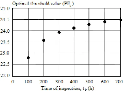
by the criterion of minimum total error probability. The plot of optimal threshold value versus time of inspection is shown in Fig. 2. As seen, the optimal threshold value increases with increasing inspection time, which is due to the increase of mathematical expectation of the random process (24) with time. Assuming k = 4, t4 = 400 h and t5 = 500 h,
the plot of the total error probability versus threshold PF4 is
shown in Fig. 3. As seen, the optimal threshold value is 24.13 kV and ()min
= 0.013. Note that if
PFi = FF = 25 [image:6.595.47.245.393.539.2]kV (i = 1, …, 4), the total error probability is 0.103. Thus, the use of the optimal replacement thresholds significantly reduces the total error probability.
Fig. 2. Optimal threshold value versus time of inspection tk (k = 1, …, 7).
Fig. 3. Total error probability versus threshold PF4 when t4 = 400 h, t5 =
500 h, PF1 = 22.75 kV, PF2 = 23.6 kV, and PF3 = 23.9 kV.
VII. CONCLUSION
In this study, we have derived the equations for the probabilities of correct and incorrect decisions when checking suitability of a stochastically deteriorating system, which is periodically inspected by imperfect measuring equipment. Proposed expressions also consider the decisions taken at the previous inspections. The problems have been formulated for determining the optimal replacement thresholds by the criteria of maximum a posteriori probability, minimum Bayes risk and minimum total error probability. The proposed general expressions for the probabilities of correct and incorrect decisions have been illustrated by the derivation of the probabilities for a monotonically increasing stochastic process. In the numerical example, the effectiveness of the proposed approach to the determination of the optimal replacement thresholds has been illustrated.
REFERENCES
[1] M. Berrade, A. Cavalcante and P. Scarf, “Maintenance scheduling of a protection system subject to imperfect inspection and replacement”,
European J. of Operational Research, vol. 218, pp.716-725, 2012. [2] V. Ulansky, "Optimal maintenance policies for electronic systems on
the basis of diagnosing", Collection of Proceedings: Issues of Technical Diagnostics. Rostov-on-Don: RISI Press, 1987, pp.137-143 (in Russian).
[3] V. Ulansky, “Trustworthiness of multiple-monitoring of operability of non-repairable electronic systems”, Collection of Proceedings: Saving Technologies and Avionics Maintenance of Civil Aviation Aircrafts. Kiev: KIIGA Press (in Russian), 1992, pp. 14-25. [4] M. Newby and R. Dagg, "Optimal inspection policies in the presence
of covariates", In: Proc. of the European Safety and Reliability Conf. ESREL’02, Lyon, 19-21 March, 2002, pp. 131-138.
[5] G. Whitmore, "Estimating degradation by a Wiener diffusion process subject to measurement error", Lifetime Data Analysis, vol. 1, 1995, pp. 307-319.
[6] M. Kallen and J. Noortwijk, "Optimal maintenance decisions under imperfect inspection", Reliability Engineering and System Safety, vol. 90 (2-3), 2005, pp. 177-185.
[7] M. Hosseini, R. Kerr and R. Randall, “An inspection model with minimal and major maintenance for a system with deterioration and Poisson failures”, IEEE Trans. Reliability, vol. 49(1), pp. 88–98, 2000.
[8] A. Ghasemia, S. Yacouta and M. Oualia, "Optimal condition based maintenance with imperfect information and the proportional hazards model", Int. J. of Production Research, vol. 45, is. 4, pp. 989-1012, 2007.
[9] A. Raza and V. Ulansky, “Modeling of discrete condition monitoring for radar”, In Proc. IEEE Microwaves, Radar and Remote Sensing Symposium, Kiev, 23-25 September, 2014, pp. 88-91.
[10] A. Buravlev, B. Dotsenko and I. Kazakov, Managing Technical Condition of Dynamic Systems. Moscow: Mashinostroenie, 1995, p. 239 (in Russian).
[11] C. Ma, Y. Shao and R. Ma, "Analysis of equipment fault prediction based on metabolism combined model", J. of Machinery Manufacturing and Automation, vol. 2, is. 3, pp. 58-62, Sept. 2013. [12] E. Ventsel and L. Ovcharov. Applied Problems of Probability Theory.
Moscow: Radio i Svyaz, 1987 (in Russian).
[13] B. Levin, Theoretical Foundations of Statistical Radio Engineering. Moscow: Soviet Radio, 1974, vol. 1, p. 141 (in Russian).
[image:6.595.49.256.559.749.2]