General features of experiments on the dynamics of laser driven electron–positron beams

(1)

General features of experiments on the dynamics of

laser-driven electron-positron beams

J. R. Warwicka, A. Alejoa, T. Dzelzainisa, W. Schumakerb, D. Doriaa, L. Romagnanic_{, K. Poder}d_{, J. M. Cole}d_{, M. Yeung}a_{, K. Krushelnick}e_{, S. P. D.} Manglesd_{, Z. Najmudin}d_{, G. M. Samarin}a_{, D. Symes}f_{, A. G. R. Thomas}e,g_,

M .Borghesia, G. Sarria

a_{School of Mathematics and Physics, Queen’s University Belfast, University Road,} Belfast, BT7 1NN, UK

b_{SLAC National Accelerator Laboratory, Menlo Park, California 94025, USA} c_{LULI, Ecole Polytechnique, CNRS, CEA, UPMC, 91128 Palaiseau, France} d_{The John Adams Institute for Accelerator Science, Blackett Laboratory, Imperial}

College London, London SW72BZ, UK

e_{Center for Ultrafast Optical Science, University of Michigan, Ann Arbor, Michigan} 481099-2099, USA

f_{Central Laser facility, Rutherford Appleton Laboratory, Didcot, Oxfordshire OX11 0QX,} UK

g_{Lancaster University, Lancaster LA1 4YB, United Kingdom}

Abstract

The experimental study of the dynamics of neutral electron-positron beams is an emerging area of research, enabled by the recent results on the genera-tion of this exotic state of matter in the laboratory. Electron-positron beams and plasmas are believed to play a major role in the dynamics of extreme astrophysical objects such as supermassive black holes and pulsars. For in-stance, they are believed to be the main constituents of a large number of astrophysical jets, and they have been proposed to significantly contribute to the emission of gamma-ray bursts and their afterglow. However, despite extensive numerical modelling and indirect astrophysical observations, a de-tailed experimental characterisation of the dynamics of these objects is still at its infancy. Here, we will report on some of the general features of ex-periments studying the dynamics of electron-positron beams in a fully laser-driven setup.

Keywords: electron-positron plasmas, proton radiography, laser wakefield acceleration

(2)

PACS: 52.27.Ep, 52.35.Qz, 52.38.Kd

1. Introduction

Pair-plasmas represent a unique state of matter, since they consist of neg-atively and positively charged particles bearing the same mass and (absolute) charge. These objects have recently been gathering increasing interest in the academic community, not only for their unique properties (see for instance, Ref. [1]) but also for the major role they play in the dynamics of a wide range of extreme astrophysical objects. For instance, magnetized electron-positron plasmas exist in pulsar magnetospheres [2], in bipolar outflows in active galactic nuclei [3], at the center of our own galaxy [4], and in the early universe [5].

Different schemes have been proposed to generate neutral pair plasmas in the laboratory. The first generation of a pair-plasma was achieved by Oohara and collaborators [6] by creating equal distributions of positively and negatively charged fullerene ions. Interestingly, this scheme allows for the long-term study of pair plasma dynamics, without having to deal with mutual annihilation, the main fundamental factor limiting the lifetime of an electron-positron plasma. More recently, active research is carried out in producing and confining low-energy populations of electrons and positrons. Whilst Penning traps can guarantee excellent confinement of either popu-lation, simultaneous confinement of both species beyond their Debye length cannot be achieved [7]. A solution to this problem has been identified in using toroidal magnetic fields either produced by levitated dipole configurations [8] or stellarators [9], as in the APEX project [10].

(3)

The structure of the paper is as follows: in Section 2 we will discuss the general features of a typical experimental setup adopted in this class of exper-iments. In section 3, we will show how the laser-driven generation of EPBs simultaneously provides an efficient way of ionising the gas through which the EPB itself is to propagate. In Section 4 we will discuss the main concepts behind detecting EPB transverse instabilities using proton radiographic tech-niques while in Section 5 we will show some typical experimental results in this area. Finally in Section 6 we will discuss some limiting factors in directly detecting density modulations in a perturbed EPB while conclusive remarks will be presented in Section 7.

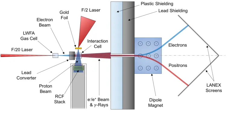
[image:3.612.118.494.331.521.2]

2. Experimental Setup

Figure 1: Typical experimental setup for the study of the dynamics of laser-driven EPBs

(4)

positrons, and gamma-ray photons [15]. Numerical and experimental work has demonstrated that the percentage of positrons in the generated EPB can be seamlessly tuned from 0% all the way up to 50% by simply changing the thickness of the solid target [14]. Typical optimum parameters of the EPB at the source thus far include a source size ofD0 '200−300µm, a duration in the range of τ '10s to 100s of fs, a number of leptons of the order of

N ' 109 _{- 10}10_{, and an average divergence of} _θ _'₃₀₋_{50 mrad. The broad} spectrum of the EPB, virtually insensitive to the initial shape of the electron spectrum but mainly determined by the cascade itself, is well approximated by a Juttner-Synge distribution, with a typical average Lorentz factor of

γ ' 10−20 [14, 15, 17]. At the source, one can easily achieve a number density of the EPB of the order of 1016 cm−3. However, due to the intrinsic energy-dependent divergence introduced by the cascade, this density drops quickly during the EPB propagation. Nonetheless, it is interesting to note that the possibility of exciting collective modes in the EPB is mostly dictated by the number of skin depths that are contained in it, either longitudinally or transversally. In the transverse direction, the number of skin depths (`S)

within the beam diameter is not influenced by the diameter (D⊥) of the

beam itself, since it can be expressed as: D⊥/`S ≈ 4.1×10−4 p

N/(γτ[fs]) [14], justifying the assumption that transverse collective behaviour is, in a first approximation, not influenced by the divergence of the beam. However, one must take into account that the broad spectrum of the EPB induces significant temporal spreading of the beam. This effectively is the main factor in determining the loss of transverse collective behaviour in the EPB as it propagates.

Several theoretical works reported in the literature (see, as possible ex-amples, Ref. [14, 19, 20, 21, 22]) have shown how the propagation of an EPB in a background electron-ion plasma might trigger the onset of a se-ries of instabilities, the most important ones namely being the oblique, the two-stream, and the filamentation (sometimes loosely referred to as Weibel) instabilities. The competition between these instabilities is ruled by a series of beam and background plasma parameters, with the dominant one arguably being the ratio between the beam densitynb and background plasma density np: α=nb/np. As a rule of thumb, oblique instabilities dominate forα1

whilst the filamentation instability dominates for α ≥1 [14, 19, 20, 21, 22]. Two-stream instabilities are instead dominant for non-relativistic beams [20] and will not be considered here.

(5)

spatial modulation of the electron and positron populations in the EPB, the generation of strong magnetic fields, and changes in the spectral shape of the EPB. However, the latter is to be expected only if the EPB is of sufficient length so that collective behaviour in the longitudinal direction can be triggered. This is not the case for experimental results reported in the literature [14, 17] and it is generally not easy to achieve this condition with current laser systems. Even though it might be possible to achieve collective behaviour in the longitudinal direction in the near future, we will not discuss it here. In the following sections, we will discuss the main experimental implications in measuring these quantities, after having discussed how the background gas gets effectively ionised after the interaction of the primary electron beam with the solid target.

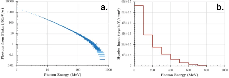
[image:5.612.112.497.361.492.2]

3. Ionisation of the background gas

Figure 2: Details of the hydrodynamic simulation used to estimate the initial conditions of the gas in the second gas cell. (a) Gamma-ray spectrum at the exit of the Pb converter, as obtained from FLUKA simulations. (b) Input used in the Hyades simulation, after binning and conversion of the spectrum in (a) to suitable units (see text for details).

(6)

[image:6.612.115.497.269.492.2]

gas, and for typical experimental parameters, it is straightforward to achieve full ionisation, with typical electron temperatures of the order of 10s of eV. This conclusion is inferred from simulations performed using HYADES [25], a commercial 1-D hydrodynamics Lagrangian code frequently used to estimate the conditions of a plasma in laboratory astrophysical studies (for examples, see Refs. [26, 27]). As an example, we will discuss the experimental conditions presented in a recent publication [17]. The simulation considers aγ-ray flash propagating through a 1 cm region filled with He gas at a backing pressure of 200 mbar.

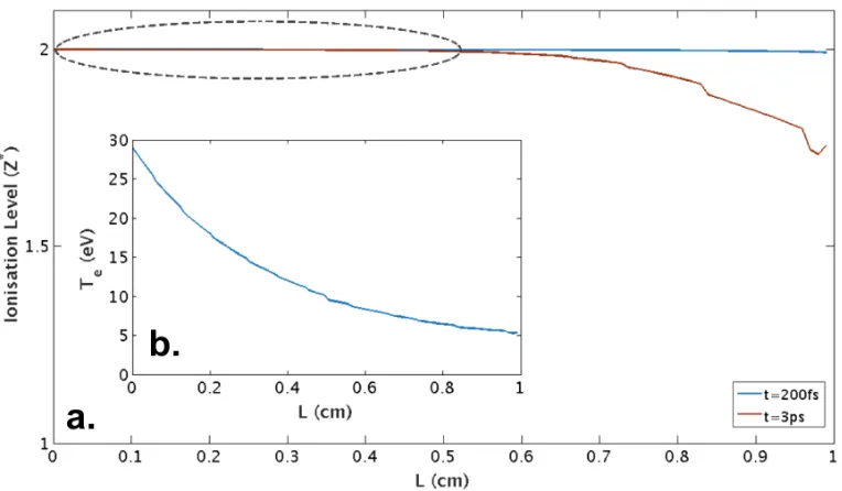
Figure 3: Results from hydrodynamic simulations on ionisation of the He gas in the second gas-cell, assuming a photon angular spectrum derived from FLUKA simulations. The ionisation level of the background gas as a function of length in the gas-cell is shown in (a), with the grey ellipse indicating the length over which the plasma is fully ionised. Insert (b) shows the related electron temperature.

(7)

that could be simulated, the energy range is divided into 100 MeV bins (or

photon group sources in HYADES nomenclature). The flux in each bin was calculated in units of erg/keV/s/cm2, as required by the code, using the equation

F = E(erg)

∆E(keV)τ(s)A(cm2₎ (1)

where E(erg) is the total energy of the photons in a bin (calculated from the spectrum obtained using FLUKA, dN_dE, as R_E0E1EdN_dEdE), ∆E(keV) is the width of the energy bin in keV, τ(s) is the duration of the gamma flash in s, and A(cm2_{) is the beam size at the entrance of the gas cell in cm}2_{. The final} calculated input is shown in Fig. 2.b.

A period of 3 ps is simulated, with variable time steps internally calculated by the code taking into account the relevant time scales of the simulation. The propagation of the gamma flash results in a prompt ionisation within the gas-cell with a plasma temperature of the order of 10 - 20 eV, as shown in Fig. 3

4. Detection of magnetic fields

Several numerical works reported in the literature indicate the onset of transverse filamentation in the beam, after propagating through a neutral background plasma. Without going in the details of the specific mechanisms involved (see, for instance, Ref. [22], for details), it will suffice to note here that transverse modulations in the EPB result in localised current in the oth-erwise overall neutral beam. These beamlets of alternating current generate azimuthal fields that co-propagate with the EPB. Due to the fast time-scales involved the EPB is only 10s to 100s of fs long and it is ultrarelativistic -it is indeed extremely challenging to detect these fields directly in the EPB; however, these fields can be transferred to the background plasma, where their detection is less problematic. A necessary condition for magnetisation of the background plasma is that the electron gyroradius be smaller than the typical scale of the magnetic field. In the EPB filamentation process, the magnetic field will grow with a spatial scale comparable to the skin depth of the beam whereas, in the non-relativistic limit, the electron gyroradius in the background plasma can be expressed as: rg = mevth/eB, where vth is

(8)

plasma gets then magnetised if the magnetic field B and the background plasma density nb obey the condition:

ξ = 5×108B[T]

r _γ

nb[cm

−3

] >1. (2)

For the parameters in Ref. [17] we obtain ξ ' 50, fully justifying the as-sumption of the background plasma being magnetised. Once deposited in the background plasma, the magnetic field will decay either via collision-less pro-cesses (if the scale is comparable to the skin depth of the background plasma) [29] or collisionally (scales much larger than the skin depth of the background plasma). The latter situation effectively corresponds to α 1. In the case of collisional decay, the typical time scales involved would be proportional to the classical conductivity of the plasma [17]; for typical experimental pa-rameters, magnetic fields can then persist for hundreds of nanoseconds up to microseconds, a comfortable timescale to measure in current laser-plasma experimental setups.

(9)

[image:9.612.180.439.132.410.2]

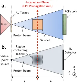
Figure 4: Sketch demonstrating how the experimental proton radiography setup (shown in a.) is simulated by the Particle Tracing code (shown in b.), with the same distances

for source-to-interaction plane, l, and interaction plane-to-detector, L. This allows for

accurate 1:1 cross-comparison between the proton signal recorded on RCF and the 2-dimensional proton density pattern yielded from PT.

signal is recorded in the form of 2-dimensional proton density maps. The high degree of laminarity of the beam implies that the real source size of the protons, usually of the order of tens of microns, is equivalent to a much narrower virtual source size of the order of a few microns [33]. The typical spatial resolution of the diagnostic then results from the interplay between the size of the proton virtual source and the resolution of the proton detector. Moreover, the laminarity of the beam ensures a geometrical magnification of the phenomenon under interest of the detector [30]:

M ≈ L+l

l (3)

(10)

and L is the distance between the interaction plane and the detector (as shown in Fig. 4). In the experiment reported in Ref. [17], l = 8 mm, and

L= 56 mm, resulting in a magnification of M ≈8.

The broadband spectrum of the laser-driven protons implies that differ-ent spectral slices in the beam will traverse the region of interest at differdiffer-ent times. The multi-layer arrangement of the RCF stack thus allows for a tem-poral multi-frame capability, even in a single shot. This is because different spectral bands will deposit most of their energy in the RCF layer that is in correspondence to the related Bragg peak. The main factors dictating the temporal resolution of each image are then: the proton pulse duration (usually in the range of a fraction of a picosecond up to a few picoseconds, de-pending on the parameters of the laser driving the protons) and the spread of energies deposited in each single RCF layer (usually of the order of ±

0.5 MeV). For low energy protons, the latter usually dominates, leading to temporal uncertainties from a few to tens of picoseconds.

In principle, this radiographic technique can be affected by a series of fac-tors, namely: the shot-to-shot fluctuation in spectral and spatial properties of the proton beam and the presence of gas-filling through which the proton beam must propagate. However, a change in spectral distribution is not im-portant, since each RCF would be sensitive, in a first approximation, to the protons whose Bragg peak lies within the position of the RCF layer within the stack [30]. Any subtle spectral effect on the radiographs is anyway taken into account on a shot-to-shot basis. Moreover, using a relatively thick and high-Z target for generating the proton beam guarantees a smooth spatial distribution in each spectral region. Finally, the presence of the gas-fill has a negligible effect on the properties of the proton beam. In order to support this statement, we have performed simulations of the scattering induced by the gas-fill on the proton beam using the commercial Monte-Carlo scattering code SRIM [34]. These simulations provide an accurate estimate of the lat-eral straggling experienced by the protons due to scattering within the gas. Simulations indicate an induced broadening of the proton beam due to the presence of a 1cm thick gas-fill at a pressure of 200 mbar of approximately 2 micron (5 micron) for a 3.3 MeV (1.1 MeV) proton at the rear side of the gas-cell. This uncertainty is smaller than the intrinsic spatial resolution of the radiographs (of the order of 10 microns), and can thus neglected in the data analysis.

(11)

the proton radiography setup used in the experiment, as illustrated in Fig. 4. The code simulates the trajectories of a laminar beam of protons, from a virtual point source, through a 3-dimensional and time-dependent electro-magnetic field distribution, to the detector plane. The proton trajectories for a defined initial energy, εp, are calculated by solving the non-relativistic

equation of motion (Eqn. 4)

d~vp dt =

e mp

(E~ +~vp×B~) (4)

where ~vp is the proton velocity, e is the elementary charge, mp is proton

mass, E~ is the electric field, andB~ is the magnetic field. The PT code traces the proton propagation to the detector plane, where it produces a simulated 2-dimensional proton density map, that can be compared with the physical data. The 3-D electromagnetic field distribution, size, and strength within the interaction region can be altered and fine-tuned until a satisfactory match is achieved.

5. Typical experimental results

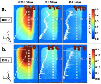
As an example of using the proton radiography technique discussed in the previous section in this class of experiments, we show in Fig. 5 radiographs of the background plasma when a quasi-neutral (row a.) or a considerably non-neutral (frame b.) beam propagates through it. The data recorded via proton radiography shows that, as the EPB composition changed from a non-neutral beam to a quasi-neutral beam, the proton signal becomes progressively more perturbed, with a distinct observable modulation when quasi-neutrality is reached. Qualitatively, this is the first experimental indication that the gen-eration and persistence of magnetic fields take place only for a quasi-neutral EPB.

In order to extract quantitative information about the magnetic fields responsible for such proton perturbations, a particle tracing (PT) code was employed. The data presented in this article refer to the same experimental parameters reported previously [17]. The best match was found for a pure magnetic field with a distribution as shown in Fig. 6. (frames a.2. and b.2.), and modelled within the PT code by Eqn. 5.

(12)

[image:12.612.110.497.128.449.2]

Figure 5: Proton radiographs of the background plasma after the propagation of a

quasi-neutral EPB with 48% e+ _{population in row (a.), and a non-neutral EPB with 23% e}+

population in row (b.). Different columns correspond to different proton energies, and therefore, different probe times after the passage of the EPB (as labelled). Each row corresponds to a single shot, highlighting the multi-frame capability of this radiographic technique. The colour-bars represent the optical density on the RCFs for the respective rows, with a higher number corresponding to higher proton density). Lineouts (white solid line) are taken from the regions between the white-dashed lines. For an EPB with 23%

e+ population (row b.), no clear modulation is seen on the proton radiographs (smooth

monotonically decreasing profile, corresponding to the initial proton beam distribution).

A pronounced modulation is observed for an EPB with 48% e+ population (row a.). The

modulation can be seen on all three layers of RCF indicating that the magnetic fields responsible for modulation are long-lived within the background plasma

where Bpeak is the peak magnetic field,ρ = p

(13)

ρf is the typical spatial scale of the magnetic field, andDbeam is the diameter

[image:13.612.113.501.199.401.2]

of the magnetic field distribution. These magnetic field distributions are azimuthal around the EPB propagation axis, which is in the z-direction, from right to left on the RCFs, as shown in Fig. 6.

Figure 6: PT results for two separate shots taken with a quasi-neutral EPB (e+_population

of 48±5%). Frames a.1. and b.1. show the raw experimental data converted to optical

density, with the spatial scale referring to the interaction plane within the background plasma. The EPB propagation direction is from right to left as indicated on the RCF. The white dashed lines show the position at which lineouts where taken on the RCFs, and after background subtraction, are plotted in frames a.3. and b.3., both in raw format (blue dotted lines) and with moving average (black dashed lines) for easier reading. Using the magnetic field distributions shown in frames a.2. and b.2. within the PT code, it was possible to extract lineouts (red dashed lines) that closely matched the experimental lineouts.

(14)

amplitude of 1.8 ± 0.2 T, with a spatial scale of ρf = 1.4 ± 0.1 mm, whilst

the radiograph in frame b. was found to be best replicated by a magnetic field distribution with peak amplitude of 1.5±0.3 T, with a spatial scale ofρf =

1.5 ± 0.1 mm. These values are consistent with those reported previously [17], confirming the robustness of the phenomenon and its detection, virtually unaffected by shot-to-shot fluctuations.

6. Direct measurements of spatial density modulations in the EPB

(15)

Given that, in the ultra-relativistic case, typical particle detectors are virtu-ally insensitive to the sign of the charge of the particle impinging on it (≤2% difference [35]), they would then not be able to display non-uniformities in the charge distribution of the beam, but only show the number density, which is kept constant even in the case of filamentation. From these simple consid-erations, one can then argue that the most suitable measurable to indicate onset of transverse instabilities in the EPB is the magnetic field left in the background plasma.

7. Conclusions

In this article, we have discussed some of the key experimental issues con-cerning the detection of instabilities experienced by a laser-driven electron-positron beam as it propagates through a background electron-ion plasma, in conditions of relevance to the dynamics of pair-dominated astrophysical scenarios such as astrophysical jets and pulsar atmospheres. According to recently published experimental results in this area, we identify the mag-netic fields left in the background plasma as the most suitable indicator of the onset of transverse instabilities and we have discussed some of the main characteristics of the detection of these fields via proton radiography.

8. Acknowledgments

The authors wish to acknowledge support from EPSRC (grants: EP/N022696/1, EP/N027175/1, EP/L013975/1, EP/N002644/1,and EP/P010059/1). The authors would also like to thank the staff at CLF for their technical support.

9. References

References

[1] E. V. Stenson et al., J. Plasma Phys. 83, 595830106 (2017) and refer-ences therein.

(16)

also various articles in Pulsars: Problems and Progress , edited by S. Johnston, M. A. Walker, and M. Bailes, Astrophysical Society (ASP) of the Pacific Conference Series 105 (ASP, San Francisco, 1996); F. C. Michel, Rev. Mod. Phys. 54 , 1 (1982).

[3] H. R. Miller and P. J. Witta, Active Galactic Nuclei (Springer-Verlag, Berlin, 1987), p. 202; M. C. Begelman, R. D. Blandford, and M. D. Rees, Rev. Mod. Phys. 56 , 255 (1984).

[4] M. L. Burns, Positron-Electron Pairs in Astrophysics , edited by M. L. Burns, A. K. Harding, and R. Ramaty (American Institute of Physics, New York, 1983), p. 281.

[5] G. W. Gibbons, S. W. Hawking and S. Siklos, The Very Early Universe (Cambridge University Press, Cambridge, 1983).

[6] W. Oohara and R. Hatakeyama, Phys. Rev. Lett. 91 , 205005 (2003); W. Oohara, D. Date and R. Hatakeyama, Phys. Rev. Lett. 95 , 175003 (2005); R. Hatakeyama and W. Oohara, Phys. Scr., 116 , 101 (2005).

[7] T.S. Pedersen et al., New J. Phys. 14, 35010 (2012).

[8] Z. Yoshida et al., Phys. Rev. Lett. 104, 235004 (2010); A.C. Boxeret al., Nat. Phys. 6, 207 (2010).

[9] Stellarator and Heliotron Devices, M. Wakatani, Oxford (1998).

[10] G. Andresen et al., Phys. Rev. Lett. 98, 023402 (2007).

[11] H. Chen et al., Phys. Rev. Lett. 114, 215001 (2015).

[12] E. Liang et al., Sci. Reports 5, 13968 (2015).

[13] G. Sarri et al., Phys. Rev. Lett. 110, 255002 (2013).

[14] G. Sarri et al., Nat. Comm. 6, 6747 (2015).

[15] G. Sarri et al., Plasma Phys. Contr. F. 55, 124017 (2013).

[16] G. Sarri et al., Plasma Phys. Contr. F. 59, 014015 (2017).

(17)

[18] E. Esarey et al., Rev. Mod. Phys. 81, 1229 (2009).