Water bodies' mapping from Sentinel 2 imagery with Modified Normalized Difference Water Index at 10 m spatial resolution produced by sharpening the swir band

remote sensing

Article

Water Bodies’ Mapping from Sentinel-2 Imagery

with Modified Normalized Difference Water Index at

10-m Spatial Resolution Produced by Sharpening the

SWIR Band

Yun Du1,*, Yihang Zhang1,2,3, Feng Ling1,4, Qunming Wang3, Wenbo Li5and Xiaodong Li1

1 _{Institute of Geodesy and Geophysics, Chinese Academy of Sciences, Wuhan 430077, China;} [email protected] (Y.Z.); [email protected] (F.L.); [email protected] (X.L.) 2 _{University of Chinese Academy of Sciences, Beijing 100049, China}

3 _{Lancaster Environment Center, Faculty of Science and Technology, Lancaster University,} Lancaster LA1 4YQ, UK; [email protected]

4 _{School of Geography, University of Nottingham, University Park, Nottingham NG7 2RD, UK}

5 _{Hefei Institute of Technology Innovation, Hefei Institutes of Physical Science, Chinese Academy of Sciences,} Hefei 230088, China; [email protected]

* Correspondence: [email protected]; Tel.: +86-27-6888-1352

Academic Editors: Clement Atzberger and Prasad S. Thenkabail

Received: 29 December 2015; Accepted: 18 April 2016; Published: 22 April 2016

Abstract:Monitoring open water bodies accurately is an important and basic application in remote sensing. Various water body mapping approaches have been developed to extract water bodies from multispectral images. The method based on the spectral water index, especially the Modified Normalized Difference Water Index (MDNWI) calculated from the green and Shortwave-Infrared (SWIR) bands, is one of the most popular methods. The recently launched Sentinel-2 satellite can provide fine spatial resolution multispectral images. This new dataset is potentially of important significance for regional water bodies’ mapping, due to its free access and frequent revisit capabilities. It is noted that the green and SWIR bands of Sentinel-2 have different spatial resolutions of 10 m and 20 m, respectively. Straightforwardly, MNDWI can be produced from Sentinel-2 at the spatial resolution of 20 m, by upscaling the 10-m green band to 20 m correspondingly. This scheme, however, wastes the detailed information available at the 10-m resolution. In this paper, to take full advantage of the 10-m information provided by Sentinel-2 images, a novel 10-m spatial resolution MNDWI is produced from Sentinel-2 images by downscaling the 20-m resolution SWIR band to 10 m based on pan-sharpening. Four popular pan-sharpening algorithms, including Principle Component Analysis (PCA), Intensity Hue Saturation (IHS), High Pass Filter (HPF) andÀ Trous Wavelet Transform (ATWT), were applied in this study. The performance of the proposed method was assessed experimentally using a Sentinel-2 image located at the Venice coastland. In the experiment, six water indexes, including 10-m NDWI, 20-m MNDWI and 10-m MNDWI, produced by four pan-sharpening algorithms, were compared. Three levels of results, including the sharpened images, the produced MNDWI images and the finally mapped water bodies, were analysed quantitatively. The results showed that MNDWI can enhance water bodies and suppressbuilt-up features more efficiently than NDWI. Moreover, 10-m MNDWIs produced by all four pan-sharpening algorithms can represent more detailed spatial information of water bodies than 20-m MNDWI produced by the original image. Thus, MNDWIs at the 10-m resolution can extract more accurate water body maps than 10-m NDWI and 20-m MNDWI. In addition, although HPF can produce more accurate sharpened images and MNDWI images than the other three benchmark pan-sharpening algorithms, the ATWT algorithm leads to the best 10-m water bodies mapping results. This is no necessary positive connection between the accuracy of the sharpened MNDWI image and the map-level accuracy of the resultant water body maps.

Remote Sens.2016,8, 354 2 of 19

Keywords:remote sensing; Modified Normalized Difference Water Index (MNDWI); Normalized Difference Water Index (NDWI); Sentinel-2; Shortwave-Infrared (SWIR); pan-sharpening; water body mapping

1. Introduction

As an important part of the Earth’s water cycle, land surface water bodies, such as rivers, lakes and reservoirs, are irreplaceable for the global ecosystem and climate system. Surveying land surface water bodies and delineating their spatial distribution has a great significance to understanding hydrology processes and managing water resources [1–3]. At present, remote sensing has become a routine approach for land surface water bodies’ monitoring, because the acquired data can provide macroscopic, real-time, dynamic and cost-effective information, which is substantially different from conventionalin situmeasurements [4–6]. Various methods, including single band density slicing [7], unsupervised and supervised classification [8–11] and spectral water indexes [12–19], were developed in order to extract water bodies from different remote sensing images. Among all existing water body mapping methods, the spectral water index-based method is a type of reliable method, because it is user friendly, efficient and has low computational cost [20]. Different water indexes have already been proposed in the past few decades. Specifically, McFeeters (1996) proposed the Normalized Difference Water Index (NDWI) [21], using the green and Near Infrared (NIR) bands of remote sensing images based on the phenomenon that the water body has strong absorbability and low radiation in the range from visible to infrared wavelengths. NDWI can enhance the water information effectively in most cases, but it is sensitive to built-up land and often results in over-estimated water bodies. To overcome the shortcomings of NDWI, Xu (2006) developed the Modified Normalized Difference Water Index (MNDWI) [22] that uses the Shortwave Infrared (SWIR) band to replace the NIR band used in NDWI. Many previous research works have demonstrated that MNDWI is more suitable to enhance water information and can extract water bodies with greater accuracy than NDWI [12,13,22,23].

In the last few decades, MNDWI had been widely applied to produce water body maps at different scales. In practice, both the spectral information of the SWIR and green bands that are used to calculate MNDWI and the spatial resolutions of both bands directly affect the accuracy of mapped water bodies. For example, MODerate-resolution Imaging Spectroradiometer (MODIS) images have been widely used to map water bodies at both global and regional scales. Specifically, Carrollet al. produced a new global raster water mask at 250-m resolution from MODIS dataset [24]. Fenget al.used MODIS images between 2000 and 2010 to estimate the inundation changes of Poyang Lake [6]. Huanget al. monitored water surface variations using long-term MODIS data time series [25]. For regional studies, images provided by the Thematic Mapper (TM), the Enhanced Thematic Mapper Plus (ETM+) and the latest Operational Land Imager (OLI) from Landsat series satellites are popular datasets. For example, Huiet al.modelled the spatial and temporal change of Poyang Lake using multi-temporal Landsat TM and ETM+ images [15]. Duet al.extracted the water body maps at subareas over the Yangtze River Basin and Huaihe River Basin in China from Landsat OLI images [13]. Rokniet al. extracted water features and detected change using Landsat TM, ETM+ and OLI images [26]. Compared to MODIS, the Landsat TM, ETM+ and OLI images have much finer spatial resolutions (30 m) and can extract open water bodies with more explicit and accurate boundaries. However, the spatial resolution of Landsat series images is still not fine enough to identify smaller-sized open water bodies, such as narrow gutters and small pools in urban areas. By exploring remote sensing images, such as SPOT6/7, IKONOS and Quick-bird, these small-sized water bodies can be mapped. However, these fine spatial resolution images have no SWIR band, making it impossible to use the MNDWI method.

Remote Sens.2016,8, 354 3 of 19

next generation of operational products, such as land cover maps, land cover change detection maps and geophysical variables [27–29]. The Sentinel-2 images would surely be of great significance for regional water bodies’ mapping, due to its appealing properties (i.e., the 10-m spatial resolution for four bands and the 10-day revisit frequency) and the free access. As shown in Table1, the Sentinel-2 multispectral image has 13 bands in total, in which four bands (blue, green, red and NIR) have a spatial resolution of 10 m and six bands (including SWIR band) have a spatial resolution of 20 m. The MNDWI method can be applied to extract water bodies from the Sentinel-2 images, since the green and SWIR bands are included. However, it is noticed that the spatial resolutions of green and SWIR bands are at 10 m and 20 m, respectively. In this case, it is easy to produce MNDWI with the 20-m resolution, by simply upscaling the green band (Band 3) from 10 m to 20 m. However, spatial information would be lost following this scheme.

Table 1.Band spatial resolution, central wavelength and bandwidth of the Sentinel-2 image.

Band Number Spatial Resolution (m) Central Wavelength (nm) Bandwidth (nm)

B1 60 443 20

B2 10 490 65

B3 10 560 35

B4 10 665 30

B5 20 705 15

B6 20 740 15

B7 20 783 20

B8 10 842 115

B8A 20 865 20

B9 60 945 20

B10 60 1375 30

B11 20 1610 90

B12 20 2190 180

Remote Sens.2016,8, 354 4 of 19

11 to 10 m to match the 10-m green Band 3, using the information provided by directly observed 10-m Bands 2, 3, 4 and 8.

The objectives of this study are to: (1) produce 10-m MNDWI from the Sentinel-2 image by sharpening the SWIR band; (2) compare the performance of various popular pan-sharpening algorithms in producing the 10-m MNDWI; (3) evaluate the performance of the produced 10-m MNDWI in water bodies mapping by comparing it to the 10-m NDWI and the 20-m MNDWI; and (4) explore the relationship between the accuracy of the sharpened SWIR band or the sharpened MNDWI image and the map-level accuracy of the resultant water body map.

2. Study Site and Dataset

The study area in this paper is located at the Venice coastland, Italy. The city of Venice and its lagoon represent an extraordinary environment and human heritage susceptible to loss in surface elevation relative to the mean sea level [39]. The lagoon covers an area of about 550 km2_{with shallows,} tidal flats, salt marshes, islands and a network of channels, which are all sensitive to the changes of surface water bodies. Over the past 100 years, the mean sea level in Venice coastland rose about 23 cm [40], which leads to an obvious expansion of the open water bodies in the Venice coastland and an increase of flooding events, causing great inconvenience for the population and enormous damage to the cultural heritage. Therefore, it is of great interest to extract surface open water bodies and to monitor their changes in the Venice coastland.

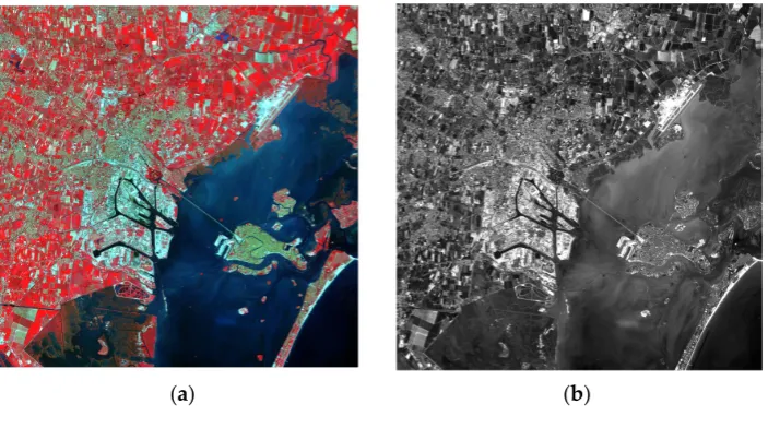
The dataset used in this study is the standard Sentinel-2 Level-1C product, which was produced by radiometric and geometric corrections, including ortho-rectification and spatial registration on a global reference system with sub-pixel accuracy. The Sentinel-2 Level-1C product is composed of 100 kmˆ100 km tiles in the UTM/WGS84 projection and provides the Top-Of-Atmosphere (TOA) reflectance. One scene of the Sentinel-2 Level-1C image acquired on 13 August 2015 (relative orbit: R022) was downloaded from the ESA Sentinel-2 Pre-Operations Hub (https://scihub.copernicus.eu/). A subset covering 20 kmˆ20 km and cantered at 45˝_{28’30”N, 12}˝_{16’29”E was used for the case study.} The false colour composite of the Sentinel-2 image at 10 m is shown in Figure1a. The study area is mainly covered by open water bodies, urban built-up and vegetation features. The images of the green band at 10 m, the NIR band at 10 m and the SWIR band at 20 m are shown in Figure1b–d, respectively, and these three bands were involved in the calculation of water indices of NDWI and MNWI.

Remote Sens. 2016, 8, 354 4 of 19

sharpening technique was chosen to increase the spatial resolution of SWIR Band 11 to 10 m to match the 10-m green Band 3, using the information provided by directly observed 10-m Bands 2, 3, 4 and 8.

The objectives of this study are to: (1) produce 10-m MNDWI from the Sentinel-2 image by sharpening the SWIR band; (2) compare the performance of various popular pan-sharpening algorithms in producing the 10-m MNDWI; (3) evaluate the performance of the produced 10-m MNDWI in water bodies mapping by comparing it to the 10-m NDWI and the 20-m MNDWI; and (4) explore the relationship between the accuracy of the sharpened SWIR band or the sharpened MNDWI image and the map-level accuracy of the resultant water body map.

2. Study Site and Dataset

The study area in this paper is located at the Venice coastland, Italy. The city of Venice and its lagoon represent an extraordinary environment and human heritage susceptible to loss in surface elevation relative to the mean sea level [39]. The lagoon covers an area of about 550 km2 _{with shallows,} tidal flats, salt marshes, islands and a network of channels, which are all sensitive to the changes of surface water bodies. Over the past 100 years, the mean sea level in Venice coastland rose about 23 cm [40], which leads to an obvious expansion of the open water bodies in the Venice coastland and an increase of flooding events, causing great inconvenience for the population and enormous damage to the cultural heritage. Therefore, it is of great interest to extract surface open water bodies and to monitor their changes in the Venice coastland.

The dataset used in this study is the standard Sentinel-2 Level-1C product, which was produced by radiometric and geometric corrections, including ortho-rectification and spatial registration on a global reference system with sub-pixel accuracy. The Sentinel-2 Level-1C product is composed of 100 km × 100 km tiles in the UTM/WGS84 projection and provides the Top-Of-Atmosphere (TOA) reflectance. One scene of the Sentinel-2 Level-1C image acquired on 13 August 2015 (relative orbit: R022) was downloaded from the ESA Sentinel-2 Pre-Operations Hub (https://scihub.copernicus.eu/). A subset covering 20 km × 20 km and cantered at 45°28′30′′N, 12°16′29′′E was used for the case study. The false colour composite of the Sentinel-2 image at 10 m is shown in Figure 1a. The study area is mainly covered by open water bodies, urban built-up and vegetation features. The images of the green band at 10 m, the NIR band at 10 m and the SWIR band at 20 m are shown in Figure 1b–d, respectively, and these three bands were involved in the calculation of water indices of NDWI and MNWI.

(a) (b)

Remote Sens.2016,8, 354 5 of 19

Remote Sens. 2016, 8, 354 5 of 19

(c) (d)

Figure 1. (a) Ten-metre false colour map (R: Band 4; G: Band 3; B: Band 8); (b) 10-m green Band 3; (c) 10-m NIR Band 8; (d) 20-m SWIR Band 11.

3. Methodology

3.1. Spectral Water Indexes

3.1.1. NDWI

The NDWI proposed by McFeeters [21] is designed to: (1) maximize the reflectance of the water body in the green band; (2) minimize the reflectance of water body in the NIR band [22,41]. McFeeters’s NDWI is calculated as:

NDWI Green NIR

Green NIR

ρ − ρ

=

ρ + ρ (1)

where ρ_Green is the TOA reflectance value of the green band and ρ_NIR is the TOA reflectance value of the NIR band. Comparing to the raw Digital Numbers (DN), TOA reflectance is more suitable in calculating NDWI [12,42,43]. The freely-available Sentinel-2 Level-1C dataset is already a standard product of TOA reflectance [27]. Therefore, no additional pre-processing is required, and the NDWI for Sentinel-2 can be directly calculated as:

3 8 10m

3 8 NDWI =ρ − ρ

ρ + ρ (2)

where ρ_{3 is the TOA reflectance of the Band 3 (the green band) of Sentinel-2 and} ρ₈ is the TOA reflectance of the Band 8 (the NIR band) of Sentinel-2. Note that both Band 3 and Band 8 of Sentinel-2 have the spatial resolution of 10 m, and thus, the calculated NDWI in Equation (2) also has the spatial resolution of 10 m. For clarity, we represent it as NDWI10m.

3.1.2. MNDWI

A main limitation of McFeeters’ NDWI is that it cannot suppress the signal noise coming from the land cover features of built-up areas efficiently [22]. Xu [22] noticed that the water body has a stronger absorbability in the SWIR band than that in the NIR band, and the built-up class has greater radiation in the SWIR band than that in the NIR band. Based on this finding, the MNDWI was proposed, which is defined as:

MNDWI Green SWIR Green SWIR

ρ − ρ

=

ρ + ρ (3)

Figure 1. (a) Ten-metre false colour map (R: Band 4; G: Band 3; B: Band 8); (b) 10-m green Band 3; (c) 10-m NIR Band 8; (d) 20-m SWIR Band 11.

3. Methodology

3.1. Spectral Water Indexes

3.1.1. NDWI

The NDWI proposed by McFeeters [21] is designed to: (1) maximize the reflectance of the water body in the green band; (2) minimize the reflectance of water body in the NIR band [22,41]. McFeeters’s NDWI is calculated as:

NDWI“ ρGreen´ρN IR

ρ_Green`ρ_{N IR} (1)

whereρ_Greenis the TOA reflectance value of the green band andρ_{N IR}is the TOA reflectance value of the NIR band. Comparing to the raw Digital Numbers (DN), TOA reflectance is more suitable in calculating NDWI [12,42,43]. The freely-available Sentinel-2 Level-1C dataset is already a standard product of TOA reflectance [27]. Therefore, no additional pre-processing is required, and the NDWI for Sentinel-2 can be directly calculated as:

NDWI10m “

ρ₃´ρ₈

ρ₃`ρ₈ (2)

where ρ₃ is the TOA reflectance of the Band 3 (the green band) of Sentinel-2 and ρ₈ is the TOA reflectance of the Band 8 (the NIR band) of Sentinel-2. Note that both Band 3 and Band 8 of Sentinel-2 have the spatial resolution of 10 m, and thus, the calculated NDWI in Equation (2) also has the spatial resolution of 10 m. For clarity, we represent it as NDWI10m.

3.1.2. MNDWI

A main limitation of McFeeters’ NDWI is that it cannot suppress the signal noise coming from the land cover features of built-up areas efficiently [22]. Xu [22] noticed that the water body has a stronger absorbability in the SWIR band than that in the NIR band, and the built-up class has greater radiation in the SWIR band than that in the NIR band. Based on this finding, the MNDWI was proposed, which is defined as:

MNDWI“ ρGreen´ρSW IR

Remote Sens.2016,8, 354 6 of 19

whereρ_{SW IR}is the TOA reflectance of the SWIR band. In general, compared to NDWI, water bodies have greater positive values in MNDWI, because water bodies generally absorb more SWIR light than NIR light; soil, vegetation and built-up classes have smaller negative values, because they reflect more SWIR light than green light [41].

For Sentinel-2, the green band has the spatial resolution of 10 m, while the SWIR band (Band 11) has the spatial resolution of 20 m. Thus, MNDWI needs to be calculated at a spatial resolution of either 10 m or 20 m. The 20-m MNDWI is calculated as:

MNDWI20m“

ρ20₃ m´ρ₁₁

ρ20₃ m`ρ₁₁ (4)

whereρ₁₁is the TOA reflectance of Band 11 (SWIR) of Sentinel-2 andρ20₃ mis the TOA reflectance of the upscaled Band 3 of Sentinel-2 with a spatial resolution of 20 m. The value ofρ20₃mis calculated as the average value of the corresponding 2ˆ2ρ₃values.

On the other hand, if the spatial resolution of Band 11 is increased from 20 m to 10 m, the MNDWI with the spatial resolution of 10 m, MNDWI10m, can then be calculated as:

MNDWI10m“

ρ₃´ρ10₁₁m

ρ₃`ρ10₁₁m (5)

whereρ10₁₁m refers to the TOA reflectance of Band 11 at 10 m, which is produced by downscaling the original 20-m Band 11. This is achieved by using the pan-sharpening algorithms described in the following.

3.2. Pan-Sharpening Algorithms

In this paper, four popular pan-sharpening algorithms, including PCA [44], IHS [45],High Pass Filter(HPF) [46] andÀ Trous Wavelet Transform(ATWT) [47] were applied to downscale the Sentinel-2 SWIR band. The basic principles of these different pan-sharpening algorithms are introduced briefly as follows.

3.2.1. PCA

PCA is an approach based on the component substitution for spectral transformation of the original data [48]. Specifically, PCA creates an uncorrelated feature space that can be used as an alternative of the data in the original multispectral feature space. The first Principal Component (PC) image with the largest variance is considered to contain the major information from the original multispectral image, and it is replaced by the fine spatial resolution PAN image [44]. It is noted that before the substitution, the histogram of the PAN image is adjusted to match the first PC. After the substitution, an inverse PC transform is performed to produce the pan-sharpened multispectral image.

3.2.2. IHS

Remote Sens.2016,8, 354 7 of 19

3.2.3. HPF

HPF is a method based on the multi-resolution analysis [34]. The general principle of HPF is to extract high frequency information that is related mostly to the spatial information from the PAN image by using a high pass filter [46]. The high frequency information is then added to each coarse band with a specified weight. Different high pass filters, including the Box filter, Gaussian and Laplacian, can be applied in HPF, and the Box filter is chosen in this paper [46].

3.2.4. ATWT

Similarly to HPF, ATWT is also based on multi-resolution analysis [34]. For ATWT, the original multispectral bands are interpolated to match the spatial resolution of the PAN band. The PAN image and each interpolated band of the multispectral image are decomposed as three high and one low frequency components through wavelet transform. The high frequency component extracted from the PAN image is then merged into the interpolated multispectral bands. Each of the pan-sharpened multispectral bands is finally obtained by the inverse wavelet transform. Three inter-band structure modes, including Context-Based Decision (CBD), Support Value Transform (SVT) and Laplacian pyramids, are widely used in ATWT to rule on the transformation of high frequency components of the PAN image [50], and the Laplacian pyramids are used in this paper.

3.2.5. Algorithm Implementation

As the pan-sharpening algorithm is based on the availability of a PAN or PAN-like band, a suitable PAN-like band needs to be selected from 10-m Bands 2, 3, 4 and 8 at first. In this study, the most suitable PAN-like band was determined by measuring the correlation coefficient between them and the SWIR band. The 10-m band with the greatest correlation coefficient is chosen as the PAN-like band [37,38].

For all four used pan-sharpening algorithms, HPF and ATWT can be applied for coarse multispectral images band by band. To produce the 10-m SWIR band with HPF and ATWT, the 20-m SIWR band can be sharpened using the PAN-like band directly. By contrast, PCA and IHS are based on the component substitution, and multiple coarse bands are required. To facilitate the implemented process, in this study, all six 20-m bands, including Bands 5, 6, 7, 8A, 11 and 12, were used in these pan-sharpening algorithms of PCA, his, HPF and ATWT.

3.3. Water Bodies’ Mapping with the OTSU Algorithm

After the NDWI or MNDWI are produced, water bodies can then be mapped by the simple segmentation algorithm using a suitable threshold value. In general, the threshold is often set to be zero in order to map water bodies from NDWI or MNDWI, that is a pixel whose NDWI or MNDWI is larger than zero is considered as water. In practice, however, multispectral images acquired by different satellite platforms at different regions and different times always have different characteristics. Thus, the threshold should be determined according to the feature of water index values themselves in each scene [51]. In this study, the OTSU algorithm [52], a widely-used dynamic threshold method aiming to maximize the inter-class variance, is employed to determine the optimal threshold valuet˚ for water bodies’ mapping with NDWI and MNDWI [12,13].

Remote Sens.2016,8, 354 8 of 19

non-water class ranging fromatotand the water class ranging fromttob. The optimal threshold valuet˚_{in the OTSU algorithm is determined as follows:}

$ ’ ’ ’ ’ & ’ ’ ’ ’ %

δ2“Pnw¨ pMnw´Mq2`Pw¨ pMw´Mq2 M“Pnw¨Mnw`Pw¨Mw

Pnw`Pw “1 t˚_{“Arg Max}

aďtďb !

Pnw¨ pMnw´Mq2`Pw¨ pMw´Mq2 )

(6)

whereδ is the inter-class variance of the non-water class and the water class, Pnm andPw are the

possibilities of one pixel belonging to non-water and water, respectively,MnwandMware the mean

values of the non-water and water classes andMis the mean value of the NDWI or MNDWI image.

3.4. Result Accuracy Assessment

In order to fully assess the performances of different methods, three levels of results, including the sharpened images, the produced MNDWI images and the final mapped water bodies, were analysed with different quantitative indexes, respectively.

TheQuality with No Reference (QNR) index that is widely used for pan-sharpening quality evaluation without reference data is employed here to assess the sharpening results [34,53]. The QNR index is calculated based on the two terms. One is the spectral distortion indexDλ, which reflects the degree of preserving the spectral information, and the other is the spatial distortion indexDs,

which reflects the degree of preserving the spatial details in the PAN band. More precisely, QNR is formulated as:

QNR“ p1´Dλqαp1´Dsqβ (7)

whereα,βare two weighted coefficients and are typically set to one. The spectral distortion indexDλ and the spatial distortion indexDsare calculated as:

Dλ“ p

g f f e

1 NpN´1q

N ÿ

i“1 N ÿ

j“1,j‰i ˇ ˇ

ˇdi,jpMS, MSfq ˇ ˇ ˇ p

(8)

Ds“ q g f f e1 N N ÿ i“1 ˇ ˇ

ˇQpMSfpiq ´Pq ´QpMS, PLRq ˇ ˇ ˇ q

(9)

wherepandqare weighted coefficients and are typically set to one.Nis the number of bands in the observed multispectral image MS, MSf is the sharpened multispectral image and PLRis upscaled from

the observed pan-like band P. TheQ´index[54] is used here to calculate the dissimilarities between bands,di,jpMS, MSfq “QpMSpiq ´MSpiqq ´QpMSfpiq ´MSfpiqq.

The value of QNR ranges from 0 to 1, and a higher QNR value indicates a more accurate sharpened result. The QNR index is designed for multiple bands (at least two bands) and cannot be used to validate the sharpened SWIR band solely. Thus, to assess the results produced by different pan-sharpening algorithms, the QNR index was calculated using the SWIR band and Band 8A.

The correlation coefficients (CC) and root-mean-square-error (RMSE) were used to quantitatively compare the four MNDWI10m images produced by four pan-sharpening algorithms. Since the real MNDWI10m image is not available, the MNDWI20m calculated by Equation (4) was used as the reference. The two indexes are calculated as:

CC“

N ř

i“1

pMNDWI20mpiq´M20mqpMNDWI10mÓ20m piq ´M 10mÓ 20m q d N ř i“1

pMNDWI20mpiq ´M20mq2¨ N ř

i“1

pMNDWI10mÓ_20m piq ´M10mÓ_20m q

Remote Sens.2016,8, 354 9 of 19

RMSE“ g f f e1

N N ÿ

i“1

pMNDWI20mpiq ´MNDWI10mÓ20m piqq2 (11)

whereNis the number of pixels in MNDWI20m, MNDWI10mÓ20m is the MNDWI image at the spatial resolution of 20 m that was generated by upscaling the sharpened MNDWI10mimages andM20mand M10mÓ20m are mean values of MNDWI20mand MNDWI10mÓ20m , respectively.

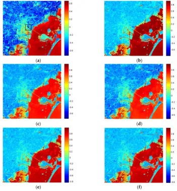
To examine the final water body maps produced with different water indexes, map-level accuracy values, including Kappa and Overall Accuracy (OA), as well as class-level accuracy values, including the omission error and the commission error, were employed. The reference water maps were produced by manually digitizing the 10-m false Sentinel-2 image with the help of Google Earth Map. As it is difficult to obtain the reference water body map for the whole study area (20 kmˆ20 km) at the spatial resolution of 10 m, the validation of the final water body maps was performed in three separate subareas, with each covering an area of 2 kmˆ2 km, as shown in Figure2a.

Remote Sens. 2016, 8, 354 9 of 19

To examine the final water body maps produced with different water indexes, map-level accuracy values, including Kappa and Overall Accuracy (OA), as well as class-level accuracy values, including the omission error and the commission error, were employed. The reference water maps were produced by manually digitizing the 10-m false Sentinel-2 image with the help of Google Earth Map. As it is difficult to obtain the reference water body map for the whole study area (20 km × 20 km) at the spatial resolution of 10 m, the validation of the final water body maps was performed in three separate subareas, with each covering an area of 2 km × 2 km, as shown in Figure 2a.

(a) (b)

(c) (d)

(e) (f)

Figure 2. (a) Ten-metre NDWI10m produced by the original green and NIR bands; (b) 20-m 20m

MNDWI (M, Modified) produced by the upscaled green band and the original SWIR band; (c) 10-m MNDWI_10mPCA produced by the original green band and the PCA-sharpened SWIR band; (d) 10-m MNDWI10mIHS produced by the original green band and the his-sharpened SWIR band;

(e) 10-m MNDWI10mHPF produced by the original green band and the High Pass Filter

(HPF)-sharpened SWIR band; (f) 10-m MNDWI10mATWT produced by the original green band and the À Trous

Wavelet Transform (ATWT)-sharpened SWIR band. The three black square frames shown in (a) indicate the locations of Subareas A, B and C, respectively.

Remote Sens.2016,8, 354 10 of 19

4. Results and Discussion

4.1. Comparison between NDWI and MNDWI

All six water indexes’ images, including NDWI10m, MNDWI20m and four 10-m MNDWI images produced by four pan-sharpening algorithms, MNDWIPCA_10m, MNDWIIHS_10m, MNDWIHPF_10m and MNDWIATWT_10m , are shown in Figure2. All NDWI and MNDWI images clearly enhance the separability of the water bodies. Most MNDWI values of water bodies are larger than 0.8, while most NDWI values of water bodies are larger than 0.5. As shown in Figure2a, NDWI values of built-up and vegetation are much different. Compared to water bodies, vegetation has much smaller NDWI values, making vegetation easy to distinguish from water bodies. However, built-up features in the NDWI image present in a light yellow tone with positive values between zero and 0.2, especially in the city centres, leading to the confusion between built-up and water bodies. Compared to NDWI, built-up features in the city areas in all MNDWI images present a light cyan tone with values below 0 (Figure2b–f), indicating that the confusion caused by built-up features in the NDWI image are notably suppressed or even removed in the MNDWI image. This phenomenon agrees with previous research results that MNDWI values of built-up would be smaller than NDWI values, because TOA reflectance values of built-up in the SWIR band are larger than those of NIR.

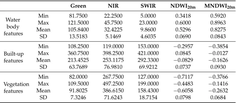
Table2lists the statistical results of water bodies, built-up and vegetation features of Band 3 (green), Band 8 (NIR), Band 11 (SWIR), NDWI and MNDWI images shown in Figure 1b–d and Figure2a,b, respectively. A similar trend shown in Figure2is also found in Table2. For water bodies, the minimum and maximum values of MNDWI are all larger than those of NDWI. The mean MNDWI value increases by about 0.3 when compared to the mean NDWI value, because the mean TOA value of the SWIR band used for MNDWI is 9.86, while the mean TOA value of the NIR band used for NDWI is 45.75. For built-up features, it is found that the maximum value of NDWI is 0.0845, which is larger than 0. If the threshold value of zero is used to segment water bodies from the NDWI image, some built-up pixels should be wrongly assigned as water. By contrast, the maximum MNDWI value of built-up features is´0.0127, which is much smaller than that of NDWI (0.0845), making built-up features easier to distinguish from water bodies.

Table 2.Maximum (Max), minimum (Min), mean and standard deviation (SD) values of water body, built-up and vegetation features within the Band 3 (green), Band 8 (NIR), Band 11 (SWIR), NDWI20m and MNDWI20mimages shown in Figure1b–d and Figure2a,b, respectively.

Green NIR SWIR NDWI20m MNDWI20m

Water body features

Min 81.7500 22.2500 5.0000 0.3418 0.5920

Max 121.5000 45.7500 23.0000 0.6000 0.8963

Mean 105.8400 32.4225 9.8600 0.5296 0.8275

SD 13.5183 5.1469 4.6035 0.0690 0.0843

Built-up features

Min 108.2500 119.0000 153.0000 ´0.2957 ´0.3854

Max 360.7500 398.2500 421.0000 0.0845 ´0.0127

Mean 213.4525 253.1175 292.3300 ´0.0829 ´0.1626

SD 63.7689 76.9810 69.9212 0.0737 0.0930

Vegetation features

Min 82.0000 267.7500 127.0000 ´0.7117 ´0.3766

Max 109.5000 497.2500 199.0000 ´0.4483 ´0.1416

Mean 91.8025 386.6150 158.4300 ´0.6058 ´0.2632

SD 7.3246 71.6243 18.7154 0.0798 0.0684

4.2. Comparison between Pan-Sharpening Results

Remote Sens.2016,8, 354 11 of 19

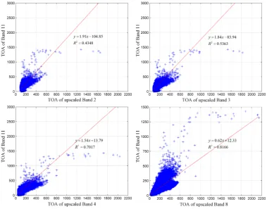
and four upscaled 20-m bands produced from the original 10-m Bands 2, 3, 4 and 8. It is noticed that Band 8 (NIR) has the greatest correction coefficient of 0.8166. Therefore, Band 8 was chosen as the PAN-like band in the pan-sharpening algorithms to produce the 10-m SWIR image.

Remote Sens. 2016, 8, 354 11 of 19

band and four upscaled 20-m bands produced from the original 10-m Bands 2, 3, 4 and 8. It is noticed that Band 8 (NIR) has the greatest correction coefficient of 0.8166. Therefore, Band 8 was chosen as the PAN-like band in the pan-sharpening algorithms to produce the 10-m SWIR image.

The QNR validation index was used to examine the sharpened SWIR bands with different pan-sharpening algorithms. Table 3 shows the QNR values, including the spectral distortion value D_λ and the spatial distortion value Ds of both sharpened bands (the SWIR band and Band 8A)

generated by PCA, IHS, HPF and ATWT, respectively. IHS has the smallest QNR value and the largest D_λ and Ds values, showing that IHS is the weakest algorithm in preserving the spectral

information of multispectral bands (20-m SWIR band and Band 8A) and the spatial detail in the PAN band (Band 8). HPF has the smallest D_λ and Ds values of 0.0843 and 0.0626, and the largest QNR

value of 0.8584, showing that HPF is more able to preserving the spectral and spatial information of the observed images. Therefore, HPF is considered as the most accurate pan-sharpening algorithm for this case.

Figure 3. Scatter maps and correlation coefficients between 20-m SWIR band and the four upscaled Bands 2, 3, 4 and 8 of Sentinel-2.

Table 3. QNR, D_λ and Ds indexes of the sharpened SWIR band and Band 8A generated by PCA, IHS, HPF and ATWT.

PCA IHS HPF ATWT

D_λ 0.1258 0.2087 0.0843 0.1342

s

D 0.1428 0.1960 0.0626 0.0872 QNR 0.7494 0.6362 0.8584 0.7902

4.3. Comparison between Different MNDWIs

In Figure 4, enlarged NDWI and MNDWI images of three subareas are shown. It is noticed that there still exists much difference among these images. In general, the spatial resolution is a significant

Figure 3.Scatter maps and correlation coefficients between 20-m SWIR band and the four upscaled Bands 2, 3, 4 and 8 of Sentinel-2.

The QNR validation index was used to examine the sharpened SWIR bands with different pan-sharpening algorithms. Table3shows the QNR values, including the spectral distortion valueDλ and the spatial distortion valueDsof both sharpened bands (the SWIR band and Band 8A) generated

by PCA, IHS, HPF and ATWT, respectively. IHS has the smallest QNR value and the largestDλ andDsvalues, showing that IHS is the weakest algorithm in preserving the spectral information of

multispectral bands (20-m SWIR band and Band 8A) and the spatial detail in the PAN band (Band 8). HPF has the smallestDλandDs values of 0.0843 and 0.0626, and the largest QNR value of 0.8584,

showing that HPF is more able to preserving the spectral and spatial information of the observed images. Therefore, HPF is considered as the most accurate pan-sharpening algorithm for this case.

Table 3.QNR,DλandDsindexes of the sharpened SWIR band and Band 8A generated by PCA, IHS, HPF and ATWT.

PCA IHS HPF ATWT

Dλ 0.1258 0.2087 0.0843 0.1342

Ds 0.1428 0.1960 0.0626 0.0872

QNR 0.7494 0.6362 0.8584 0.7902

4.3. Comparison between Different MNDWIs

Remote Sens.2016,8, 354 12 of 19

factor that affects the information of water bodies in the MNDWI image. In the NDWI20mimage, many water bodies, especially linear water features, were invisible, and many jagged squares appeared around water boundaries, due to its relatively coarse spatial resolution. By contrast, in all MNDWI10m

images, more spatial details of water bodies, especially linear water features, were represented more clearly, and water boundaries become smoother. This is because the sharpened SWIR band, which is used in producing the 10-m MNDWI images, inherited 10-m detailed spatial information from Band 8 (NIR). Visual inspection reveals that PCA- and IHS-based MNDWI images present a dark orange tone that is similar to the 10-m NDWI image, and some water bodies, especially linear water features, are not sufficiently enhanced. This is because the results of PCA and IHS rely heavily on the selected PAN-like band. Since the selected PAN-like band in this study is the 10-m NIR band, the 10-m MNDWI images produced by PCA and IHS are predictably similar to the 10-m NDWI. Compared to PCA and IHS, the ATWT and HPF MNDWI images present a darker red tone that is more similar to the original 20-m MNDWI, and water bodies are all enhanced. This is because HPF and ATWT can preserve more spectral information of the original multispectral image [34].

Remote Sens. 2016, 8, 354 12 of 19

factor that affects the information of water bodies in the MNDWI image. In the NDWI20m image, many water bodies, especially linear water features, were invisible, and many jagged squares appeared around water boundaries, due to its relatively coarse spatial resolution. By contrast, in all

10

MNDWI m images, more spatial details of water bodies, especially linear water features, were

represented more clearly, and water boundaries become smoother. This is because the sharpened SWIR band, which is used in producing the 10-m MNDWI images, inherited 10-m detailed spatial information from Band 8 (NIR). Visual inspection reveals that PCA- and IHS-based MNDWI images present a dark orange tone that is similar to the 10-m NDWI image, and some water bodies, especially linear water features, are not sufficiently enhanced. This is because the results of PCA and IHS rely heavily on the selected PAN-like band. Since the selected PAN-like band in this study is the 10-m NIR band, the 10-m MNDWI images produced by PCA and IHS are predictably similar to the 10-m NDWI. Compared to PCA and IHS, the ATWT and HPF MNDWI images present a darker red tone that is more similar to the original 20-m MNDWI, and water bodies are all enhanced. This is because HPF and ATWT can preserve more spectral information of the original multispectral image [34].

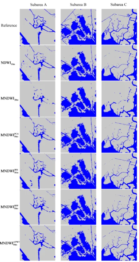
Figure 4. Subarea of the 10-m false colour maps, NDWI and MNDWI images shown in Figures 1 and 2. The first column is for Subarea A; the second column is for Subarea B; and the third column is for Subarea C.

Remote Sens.2016,8, 354 13 of 19

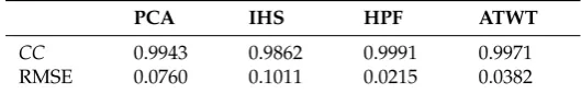
Table4shows CC and RMSE values between the original MNDWI20mimage and four MNDWI20m

images upscaled from the MNDWI10mimages produced by PCA, IHS, HPF and ATWT. The trend

of CC and RMSE is similar to that of the sharpened band validation result based on the QNR index. The MNDWI image produced by IHS has the smallest CC and the largest RMSE, and HPF produced the largest CC and the smallest RMSE, meaning that HPF has the most satisfactory performance, while IHS has the weakest performance in preserving the information within the observed 20-m MNDWI image.

Table 4. The correlation coefficient (CC) and RMSE between original MNDWI20mimage and four upscaled MNDWI10m_20mÓimages produced by PCA, HIS, HPF and ATWT.

PCA IHS HPF ATWT

CC 0.9943 0.9862 0.9991 0.9971

RMSE 0.0760 0.1011 0.0215 0.0382

4.4. Comparison between the Resulting Water Body Maps

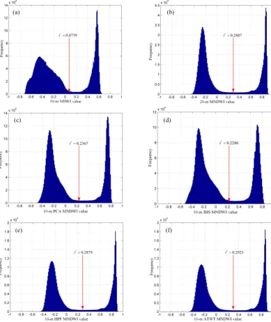
The final water body maps were extracted by segmenting the NDWI or MNDWI images with the optimal threshold valuet˚_{calculated by the OTSU algorithm. Figure5shows the histogram and} the corresponding optimal threshold value of each NDWI or MNDWI image. All histograms have bimodal shapes, and optimal threshold values calculated by the OTSU algorithm are all located at the bottoms. In general, the optimal threshold value of NDWI is much smaller than those of MNDWI. The histograms of MNDWI20m, MNDWIHPF10m and MNDWIATWT10m are similar, and their optimal threshold values are also close. The histogram peak valleys of MNDWIPCA_10m and MNDWIIHS_10mare narrower, and their optimal threshold values are smaller than those of MNDWIHPF10m and MNDWIATWT10m .

Remote Sens.2016,8, 354 14 of 19

Remote Sens. 2016, 8, 354 14 of 19

Figure 5. The histograms and optimal threshold values calculated by the OTSU method for the: (a) NDWI10m ; (b) MNDWI20m ; (c)

PCA 10m

MNDWI ; (d) MNDWI10mIHS ; (e) MNDWI10mHPF ; and (f) MNDWI_10mATWT.

The corresponding statistic accuracies of three different water body maps are shown in Table 5. Water body maps produced by 10-m NDWI images have the smallest average commission errors. When compared to MNDWI10m, however, large average omission errors are also achieved in 10-m NDWI images, because MNDWI is more suitable to enhance the water body features than NDWI.

20m

MNDWI has the largest average omission error, due to its coarse spatial resolution. Compared to

20m

MNDWI , the average Kappa values of MNDWI10m produced by PCA, IHS, HPF and ATWT are larger, showing the effectiveness of pan-sharpening for water bodies’ mapping. Compared to NDWI, the average Kappa values of MNDWI10m produced by PCA, IHS HPF and ATWT increase by 0.0262, 0.0245, 0.0065 and 0.0338, respectively. This indicates the superiority of MNDWI over NDWI. Although the average commission errors of MNDWI10mATWT are larger than those of

HPF 10m MNDWI , Figure 5. The histograms and optimal threshold values calculated by the OTSU method for the: (a) NDWI10m; (b) MNDWI20m; (c) MNDWIPCA_10m; (d) MNDWIIHS_10m; (e) MNDWIHPF_10m; and (f) MNDWIATWT_10m .

Remote Sens.2016,8, 354 15 of 19

Remote Sens. 2016, 8, 354 15 of 19

PCA 10m

MNDWI and NDWI, the largest average Kappa and OA values and the smallest average omission error are achieved by MNDWI10mATWT, suggesting the superiority of ATWT in mapping water bodies.

Figure 6. Subarea reference 10-m water body maps and 20-m and 10-m water body maps extracted from the sub-area NDWI and MNDWI images shown in Figure 4.

Table 5. Kappa, Overall Accuracy (OA), omission error and commission error of resultant water body maps in Subareas A, B and C.

10m

NDWI MNDWI20m

PCA 10m

MNDWI IHS

10m

MNDWI HPF

10m

MNDWI ATWT

10m

MNDWI

Kappa

A 0.8464 0.7037 0.8756 0.8700 0.8334 0.8846 B 0.8974 0.8579 0.8955 0.8954 0.8905 0.8971 C 0.8435 0.8289 0.8947 0.8952 0.8828 0.9070 Average 0.8624 0.7968 0.8886 0.8869 0.8689 0.8962

OA

A 97.20% 95.36% 97.78% 97.61% 97.13% 97.92% B 95.07% 93.12% 94.92% 94.91% 94.67% 94.99% C 94.86% 94.28% 96.41% 96.44% 96.02% 96.79% Average 95.71% 94.25% 96.37% 96.32% 95.94% 96.57%

A 8.81% 1.98% 3.30% 7.55% 2.74% 3.53% Figure 6.Subarea reference 10-m water body maps and 20-m and 10-m water body maps extracted from the sub-area NDWI and MNDWI images shown in Figure4.

Table 5.Kappa, Overall Accuracy (OA), omission error and commission error of resultant water body maps in Subareas A, B and C.

NDWI10m MNDWI20m MNDWIPCA10m MNDWIIHS10m MNDWIHPF10m MNDWIATWT10m

Kappa

A 0.8464 0.7037 0.8756 0.8700 0.8334 0.8846

B 0.8974 0.8579 0.8955 0.8954 0.8905 0.8971

C 0.8435 0.8289 0.8947 0.8952 0.8828 0.9070

Average 0.8624 0.7968 0.8886 0.8869 0.8689 0.8962

OA

A 97.20% 95.36% 97.78% 97.61% 97.13% 97.92%

B 95.07% 93.12% 94.92% 94.91% 94.67% 94.99%

C 94.86% 94.28% 96.41% 96.44% 96.02% 96.79%

Average 95.71% 94.25% 96.37% 96.32% 95.94% 96.57%

Commission Error

A 8.81% 1.98% 3.30% 7.55% 2.74% 3.53%

B 2.53% 7.65% 6.92% 6.87% 6.94% 7.08%

C 0.47% 4.71% 2.33% 1.92% 2.88% 2.99%

Average 3.94% 4.78% 4.18% 5.45% 4.19% 4.53%

Omission Error

A 18.29% 42.19% 17.93% 15.43% 24.68% 16.34%

B 9.54% 9.05% 5.21% 5.28% 5.81% 4.83%

C 21.89% 20.85% 13.48% 13.75% 14.72% 11.15%

Remote Sens.2016,8, 354 16 of 19

4.5. Impact of the Threshold Value on the Performance of Water Mapping

Figure7is used here to show how the threshold values affect the performance of water mapping for different NDWI and MNDWI images of different methods. The water mapping threshold value is set to be in the range of zero to 0.4 with an interval of 0.05 by considering the histograms of different NDWI and MNDWI images shown in Figure5. From Figure7, it can be found that the optimal threshold value of the NDIW image is in the range of zero to 0.1, while that of MNDWI images are in the range of 0.2 to 0.35, and the optimal threshold valuest˚_{calculated by the OTSU algorithm (see} Figure5) for NDWI and MNDWI images are following these optimal ranges of zero to 0.1 (NDWI) and 0.2 to 0.35 (MDNWI). NDWI is more sensitive to the change of the water mapping threshold value than MDNWI. If the threshold value of NDWI is larger than 0.1, the Kappa values of the resultant water maps will have a severe decrease. Similar trends shown in Table5are also found in Figure7; the MNDWI20mhas the lowest Kappa values in the optimal ranges by comparing to other 10-m NDWI and MNDWI images. For the four pan-sharpening-based 10-m MNDWI images, the results of ATWT have the highest Kappa values by comparing to those of PCA, IHS and HPF.

Remote Sens. 2016, 8, 354 16 of 19

Commission Error

B 2.53% 7.65% 6.92% 6.87% 6.94% 7.08% C 0.47% 4.71% 2.33% 1.92% 2.88% 2.99% Average 3.94% 4.78% 4.18% 5.45% 4.19% 4.53%

Omission Error

A 18.29% 42.19% 17.93% 15.43% 24.68% 16.34% B 9.54% 9.05% 5.21% 5.28% 5.81% 4.83% C 21.89% 20.85% 13.48% 13.75% 14.72% 11.15% Average 16.57% 24.03% 12.21% 11.49% 15.07% 10.77%

4.5. Impact of the Threshold Value on the Performance of Water Mapping

Figure 7 is used here to show how the threshold values affect the performance of water mapping for different NDWI and MNDWI images of different methods. The water mapping threshold value is set to be in the range of zero to 0.4 with an interval of 0.05 by considering the histograms of different NDWI and MNDWI images shown in Figure 5. From Figure 7, it can be found that the optimal threshold value of the NDIW image is in the range of zero to 0.1, while that of MNDWI images are in the range of 0.2 to 0.35, and the optimal threshold values t* calculated by the OTSU algorithm (see Figure 5) for NDWI and MNDWI images are following these optimal ranges of zero to 0.1 (NDWI) and 0.2 to 0.35 (MDNWI). NDWI is more sensitive to the change of the water mapping threshold value than MDNWI. If the threshold value of NDWI is larger than 0.1, the Kappa values of the resultant water maps will have a severe decrease. Similar trends shown in Table 5 are also found in Figure 7; the MNDWI20m has the lowest Kappa values in the optimal ranges by comparing to other 10-m NDWI and MNDWI images. For the four pan-sharpening-based 10-m MNDWI images, the results of ATWT have the highest Kappa values by comparing to those of PCA, IHS and HPF.

Figure 7. The mean Kappa values of the water maps of Subarea A, B and C produced by different water mapping threshold values (in the range of 0 to 0.4).

5. Conclusions

The newly-launched Sentinel-2 can provide fine spatial resolution multispectral imagery at a fine temporal resolution, which makes it an important dataset for water bodies’ mapping at the global scale. In this paper, a novel method is proposed for water bodies’ mapping from the Sentinel-2 image by producing the 10-m MNDWI image. In order to take full advantage of the Sentinel-2 image that has four 10-m bands, including green and NIR, and six 20-m bands, including SWIR, pan-sharpening is applied to downscale the 20-m SWIR band to 10 m by using the 10-m NIR band as the PAN-like band. Four popular pan-sharpening algorithms, including PCA, IHS, HPF and ATWT, are compared. The experiment on the subset Sentinel-2 image located at Venice coastland demonstrates that MNDWI is more efficient to enhance water bodies and to suppress built-up features than NDWI. All 10-m MNDWIs produced by PCA, IHS, HPF and ATWT can represent more detailed spatial

Figure 7.The mean Kappa values of the water maps of Subarea A, B and C produced by different water mapping threshold values (in the range of 0 to 0.4).

5. Conclusions

Remote Sens.2016,8, 354 17 of 19

However, HPF makes a confusion between water and non-water body features and cannot produce water body maps with higher accuracy than the other three pan-sharpening algorithms. Compared to PCA, IHS and HPF, ATWT is most likely to enhance water body features (especially the linear water body features) and can produce the most reliable 10-m MNDWI, which yields the most accurate water bodies’ maps. In general, this is no necessary positive connection between the accuracy (QNR, CC and RMSE values) of the sharpened SWIR band or the sharpened MNDWI image and the map-level accuracy of the resultant water body map, because the two kinds of accuracies focus on different key points. QNR, CC and RMSE aim to measure the similarity between the sharpened image and the observed coarse image, while map-level accuracy of the resultant water body map mainly focuses on the difference between water body features and non-water features in the NDWI or MNDWI images. In future research, more powerful pan-sharpening algorithms, which can better take into account the characteristics and water body feature and the spectral and spatial features of the Sentinel-2 image will be explored.

Acknowledgments:This work was supported in part by the Natural Science Foundation of Hubei Province for Distinguished Young Scholars under Grant 2013CFA031, by the National Basic Research Program (973 Program) of China under Grant 2013CB733205 and the key project from Institute of Geodesy and Geophysics under Grant Y409123012.

Author Contributions: Yun Du, Yihang Zhang and Feng Ling conceived of the main idea and designed and performed the experiments. Qunming Wang made contributions to the pan-sharpening model. Wenbo Li and Xiaodong Li made contributions to the water index models. The manuscript was written by Yun Du and Yihang Zhang and was improved by the contributions of all of the co-authors.

Conflicts of Interest:The authors declare no conflict of interest.

References

1. Papa, F.; Prigent, C.; Rossow, W.B. Monitoring flood and discharge variations in the large siberian rivers from a multi-satellite technique.Surv. Geophys.2008,29, 297–317. [CrossRef]

2. Roberts, N.; Taieb, M.; Barker, P.; Damnati, B.; Icole, M.; Williamson, D. Timing of the younger dryas event in east-Africa from lake-level changes.Nature1993,366, 146–148. [CrossRef]

3. Vorosmarty, C.J.; Sharma, K.P.; Fekete, B.M.; Copeland, A.H.; Holden, J.; Marble, J.; Lough, J.A. The storage and aging of continental runoff in large reservoir systems of the world.AMBIO1997,26, 210–219.

4. Chen, Q.L.; Zhang, Y.Z.; Ekroos, A.; Hallikainen, M. The role of remote sensing technology in the EU water framework directive (WFD).Environ. Sci. Policy2004,7, 267–276. [CrossRef]

5. Du, Y.; Xue, H.P.; Wu, S.J.; Ling, F.; Xiao, F.; Wei, X.H. Lake area changes in the middle Yangtze region of China over the 20th century.J. Environ. Manag.2011,92, 1248–1255. [CrossRef] [PubMed]

6. Feng, L.; Hu, C.M.; Chen, X.L.; Cai, X.B.; Tian, L.Q.; Gan, W.X. Assessment of inundation changes of Poyang Lake using MODIS observations between 2000 and 2010.Remote Sens. Environ.2012,121, 80–92. [CrossRef] 7. Work, E.A.; Gilmer, D.S. Utilization of satellite data for inventorying prairie ponds and lakes.

Photogramm. Eng. Remote Sens.1976,42, 685–694.

8. Sivanpillai, R.; Miller, S.N. Improvements in mapping water bodies using ASTER data.Ecol. Inform.2010,5, 73–78. [CrossRef]

9. Sheng, Y.W.; Shah, C.A.; Smith, L.C. Automated image registration for hydrologic change detection in the lake-rich Arctic.IEEE Geosci. Remote Sens. Lett.2008,5, 414–418. [CrossRef]

10. Huang, C.; Chen, Y.; Wu, J.P. DEM-based modification of pixel-swapping algorithm for enhancing floodplain inundation mapping.Int. J. Remote Sens.2014,35, 365–381. [CrossRef]

11. Huang, C.; Chen, Y.; Wu, J.P. Mapping spatio-temporal flood inundation dynamics at large river basin scale using time-series flow data and MODIS imagery.Int. J. Appl. Earth Obs. Geoinf.2014,26, 350–362. [CrossRef] 12. Li, W.B.; Du, Z.Q.; Ling, F.; Zhou, D.B.; Wang, H.L.; Gui, Y.M.; Sun, B.Y.; Zhang, X.M. A comparison of land surface water mapping using the normalized difference water index from TM, ETM plus and ALI. Remote Sens.2013,5, 5530–5549. [CrossRef]

Remote Sens.2016,8, 354 18 of 19

14. Xie, H.; Luo, X.; Xu, X.; Tong, X.H.; Jin, Y.M.; Pan, H.Y.; Zhou, B.Z. New hyperspectral difference water index for the extraction of urban water bodies by the use of airborne hyperspectral images.J. Appl. Remote Sens. 2014,8, 085098. [CrossRef]

15. Hui, F.M.; Xu, B.; Huang, H.B.; Yu, Q.; Gong, P. Modelling spatial-temporal change of Poyang Lake using multitemporal Landsat imagery.Int. J. Remote Sens.2008,29, 5767–5784. [CrossRef]

16. Jiang, H.; Feng, M.; Zhu, Y.Q.; Lu, N.; Huang, J.X.; Xiao, T. An automated method for extracting rivers and lakes from landsat imagery.Remote Sens.2014,6, 5067–5089. [CrossRef]

17. Mizuochi, H.; Hiyama, T.; Ohta, T.; Nasahara, K.N. Evaluation of the surface water distribution in north-central namibia based on MODIS and AMSR series.Remote Sens.2014,6, 7660–7682. [CrossRef] 18. Yao, F.F.; Wang, C.; Dong, D.; Luo, J.C.; Shen, Z.F.; Yang, K.H. High-resolution mapping of urban surface

water using ZY-3 multi-spectral imagery.Remote Sens.2015,7, 12336–12355. [CrossRef]

19. Li, W.; Qin, Y.; Sun, Y.; Huang, H.; Ling, F.; Tian, L.; Ding, Y. Estimating the relationship between dam water level and surface water area for the Danjiangkou Reservoir using Landsat remote sensing images. Remote Sens. Lett.2016,7, 121–130. [CrossRef]

20. Ryu, J.H.; Won, J.S.; Min, K.D. Waterline extraction from Landsat TM data in a tidal flat—A case study in Gomso Bay, Korea.Remote Sens. Environ.2002,83, 442–456. [CrossRef]

21. McFeeters, S.K. The use of the normalized difference water index (NDWI) in the delineation of open water features.Int. J. Remote Sens.1996,17, 1425–1432. [CrossRef]

22. Xu, H.Q. Modification of normalised difference water index (NDWI) to enhance open water features in remotely sensed imagery.Int. J. Remote Sens.2006,27, 3025–3033. [CrossRef]

23. Singh, K.V.; Setia, R.; Sahoo, S.; Prasad, A.; Pateriya, B. Evaluation of NDWI and MNDWI for assessment of waterlogging by integrating digital elevation model and groundwater level.Geocarto Int.2015,30, 650–661. [CrossRef]

24. Carroll, M.L.; Townshend, J.R.; DiMiceli, C.M.; Noojipady, P.; Sohlberg, R.A. A new global raster water mask at 250 m resolution.Int. J. Digit. Earth.2009,2, 291–308. [CrossRef]

25. Huang, S.F.; Li, J.G.; Xu, M. Water surface variations monitoring and flood hazard analysis in Dongting Lake area using long-term Terra/MODIS data time series.Nat. Hazards2012,62, 93–100. [CrossRef]

26. Rokni, K.; Ahmad, A.; Selamat, A.; Hazini, S. Water feature extraction and change detection using multitemporal landsat imagery.Remote Sens.2014,6, 4173–4189. [CrossRef]

27. Drusch, M.; Del Bello, U.; Carlier, S.; Colin, O.; Fernandez, V.; Gascon, F.; Hoersch, B.; Isola, C.; Laberinti, P.; Martimort, P.; et al. Sentinel-2: ESA’s optical high-resolution mission for GMES operational services. Remote Sens. Environ.2012,120, 25–36. [CrossRef]

28. Pesaresi, M.; Corbane, C.; Julea, A.; Florczyk, A.; Syrris, V.; Soille, P. Assessment of the Added-Value of Sentinel-2 for Detecting Built-up Areas.Remote Sens.2016,8, 299. [CrossRef]

29. Immitzer, M.; Vuolo, F.; Atzberger, C. First Experience with Sentinel-2 Data for Crop and Tree Species Classifications in Central Europe.Remote Sens.2016,8, 166. [CrossRef]

30. Atkinson, P.M. Downscaling in remote sensing.Int. J. Appl. Earth Obs. Geoinf.2013,22, 106–114. [CrossRef] 31. Atkinson, P.M.; Pardo-Iguzquiza, E.; Chica-Olmo, M. Downscaling cokriging for super-re solution mapping

of continua in remotely sensed images.IEEE Trans. Geosci. Remote Sens.2008,46, 573–580. [CrossRef] 32. Ashraf, S.; Brabyn, L.; Hicks, B.J. Image data fusion for the remote sensing of freshwater environments.

Appl. Geogr.2012,32, 619–628. [CrossRef]

33. Zhang, H.K.K.; Huang, B. A new look at image fusion methods from a bayesian perspective.Remote Sens. 2015,7, 6828–6861. [CrossRef]

34. Vivone, G.; Alparone, L.; Chanussot, J.; Dalla Mura, M.; Garzelli, A.; Licciardi, G.A.; Restaino, R.; Wald, L. A critical comparison among pansharpening algorithms.IEEE Trans. Geosci. Remote Sens.2015,53, 2565–2586. [CrossRef]

35. Che, X.H.; Feng, M.; Jiang, H.; Song, J.; Jia, B. Downscaling MODIS surface reflectance to improve water body extraction.Adv. Meteorol.2015,2015, 424291. [CrossRef]

36. Wu, G.P.; Liu, Y.B. Downscaling surface water inundation from coarse data to fine-scale resolution: Methodology and accuracy assessment.Remote Sens.2015,7, 15989–16003. [CrossRef]

Remote Sens.2016,8, 354 19 of 19

38. Wang, Q.M.; Shi, W.Z.; Atkinson, P.M.; Pardo-Iguquiza, E. A new geostatistical solution to remote sensing image downscaling.IEEE Trans. Geosci. Remote Sens.2016,54, 386–396. [CrossRef]

39. Strozzi, T.; Teatini, P.; Tosi, L. TerraSAR-X reveals the impact of the mobile barrier works on Venice coastland stability.Remote Sens. Environ.2009,113, 2682–2688. [CrossRef]

40. Tosi, L.; Carbognin, L.; Teatini, P.; Strozzi, T.; Wegmuller, U. Evidence of the present relative land stability of Venice, Italy, from land, sea, and space observations.Geophys. Res. Lett.2002,29, 3-1–3-4. [CrossRef] 41. Sun, F.D.; Sun, W.X.; Chen, J.; Gong, P. Comparison and improvement of methods for identifying waterbodies

in remotely sensed imagery.Int. J. Remote Sens.2012,33, 6854–6875. [CrossRef]

42. Chander, G.; Markham, B.L.; Helder, D.L. Summary of current radiometric calibration coefficients for Landsat MSS, TM, ETM+, and EO-1 ALI sensors.Remote Sens. Environ.2009,113, 893–903. [CrossRef]

43. Ko, B.C.; Kim, H.H.; Nam, J.Y. Classification of potential water bodies using landsat 8 OLI and a combination of two boosted random forest classifiers.Sensors2015,15, 13763–13777. [CrossRef] [PubMed]

44. Chavez, P.S.; Kwarteng, A.Y. Extracting spectral contrast in landsat thematic mapper image data using selective principal component analysis.Photogramm. Eng. Remote Sens.1989,55, 339–348.

45. Carper, W.J.; Lillesand, T.M.; Kiefer, R.W. The use of intensity-hue-saturation transformations for merging spot panchromatic and multispectral image data.Photogramm. Eng. Remote Sens.1990,56, 459–467. 46. Chavez, P.S.; Sides, S.C.; Anderson, J.A. Comparison of 3 different methods to merge multiresolution and

multispectral data—Landsat tm and spot panchromatic.Photogramm. Eng. Remote Sens.1991,57, 295–303. 47. Shensa, M.J. The discrete wavelet transform—Wedding the a trous and mallat algorithms. IEEE Trans.

Signal Process.1992,40, 2464–2482. [CrossRef]

48. Shah, V.P.; Younan, N.H.; King, R.L. An efficient pan-sharpening method via a combined adaptive PCA approach and contourlets.IEEE Trans. Geosci. Remote Sens.2008,46, 1323–1335. [CrossRef]

49. Huang, P.S.; Tu, T.M. A new look at IHS-like image fusion methods.Inf. Fusion2007,8, 217–218. [CrossRef] 50. Garzelli, A.; Aiazzi, B.; Alparone, L.; Baronti, S.; Nencini, F. Interband structure modeling for oversampled multiresolution analysis-based Pan-sharpening of very high resolution multispectral images.Proc. SPIE 2003,5207, 678–689.

51. Ji, L.; Zhang, L.; Wylie, B. Analysis of dynamic thresholds for the normalized difference water index. Photogramm. Eng. Remote Sens.2009,75, 1307–1317. [CrossRef]

52. Lin, K.C. On improvement of the computation speed of Otsu’s image thresholding.J. Electron. Imaging2005, 14, 023011. [CrossRef]

53. Alparone, L.; Alazzi, B.; Baronti, S.; Garzelli, A.; Nencini, F.; Selva, M. Multispectral and panchromatic data fusion assessment without reference.Photogramm. Eng. Remote Sens.2008,74, 193–200. [CrossRef]

54. Wang, Z.; Bovik, A.C. A universal image quality index.IEEE Signal Process. Lett.2002,9, 81–84. [CrossRef]