RMSE (Root Mean Square Error), respectively.



Abstract—The purposes of this research are to find a model to forecast the electricity consumption in a household and to find the most suitable forecasting period whether it should be in daily, weekly, monthly, or quarterly. The time series data in our study was individual household electric power consumption from December 2006 to November 2010. The data analysis has been performed with the ARIMA (Autoregressive Integrated Moving Average) and ARMA (Autoregressive Moving Average) models. The suitable forecasting methods and the most suitable forecasting period were chosen by considering the smallest value of AIC (Akaike Information Criterion) and RMSE (Root Mean Square Error), respectively. The result of the study showed that the ARIMA model was the best model for finding the most suitable forecasting period in monthly and quarterly. On the other hand, ARMAmodel was the best model for finding the most suitable forecasting period in daily and weekly. Then, we calculated the most suitable forecasting period and it showed that the method were suitable for short term as 28 days, 5 weeks, 6 months and 2 quarters, respectively.

Index Terms—Time Series Analysis, ARMA model, ARIMA model, R language

I. INTRODUCTION

URRENTLY, various organizations are adopting information technology to assist their jobs by providing adequate storage units to store an up to date information and used that information to the highest benefit with various methods. Planning by forecasting trends in the future is one way to apply statistical knowledge to analyze data in the past that are related to the current event. The results were used to predict future events. Time series is the order of historical data, which resembles the group or observation of the data that have been collected over time according to the continuous period of time. That collected data may already be in a daily, weekly, monthly, quarterly, or yearly format, depending on which one is appropriate to use. Time series data consist of four components: trend, seasonal effect, cyclical, and irregular effect [1]. The analysis of a time

Manuscript received December 6, 2012; revised January 10, 2013. This work was supported in part by grant from Suranaree University of Technology through the funding of Data Engineering Research Unit.

P. Chujai is a doctoral student with the School of Computer Engineering, Suranaree University of Technology, Nakhon Ratchasima 30000, Thailand (e-mail: [email protected]).

N. Kerdprasop is an associate professor with the School of Computer Engineering, Suranaree University of Technology, Nakhon Ratchasima 30000, Thailand.

K. Kerdprasop is an associate professor with the School of Computer Engineering, Suranaree University of Technology, Nakhon Ratchasima 30000, Thailand.

series used forecasting techniques to identify models from the past data. With the assumption that the information will resemble itself in the future, we can thus forecast future events from the occurred data.

There are several methods of statistical forecasting such as regressing analysis, classical decomposition method, Box and Jenkins and smooting techniques. These techniques provide forecasting models of different accuracy. The accuracy of the prediction is based on the minimum error of the forecast. The appropriate prediction methods are considered from several factors such as prediction interval, prediction period, characteristic of time series, and size of time series [2].

In this research, we are interest in time series analysis with the most popular method, that is, the Box and Jenkins method [3]. The result model of this method is quite accurate compared to other methods and can be applied to all types of data movement. There were two forecasting techniques that were used in this study; Autoregressive Integrated Moving Average (ARIMA) and Autoregressive Moving Average (ARMA). We applied these methods for detecting patterns and trends of the electric power consumption in the household with real time series period in daily, weekly, monthly, and quarterly [14]. We used program R and Rstudio [4], [5], for constructing the model [6], [7], [8]. The most suitable forecasting method and the best choice of period were chosen by considering the smallest value of AIC (Akaike Information Criterion) and RMSE(Root Mean Square Error), respectively.

The remainder of this research is organized as follow. Section 2 contains the literature review. In Section 3, we present details about the computational approach for deriving time series model. Experimental results of our analysis are given in Section 4. Finally, we conclude and discuss our future work in Section 5.

II. LITERATUREREVIEW

The current various researches have used the method of forecasting with time series data such as the electric power consumption. Saab and colleagues [9] studied the forecasting method for monthly electric energy consumption in Lebanon. They used two different univariate modeling methods namely, ARIMA and AR(1) with a highpass filter. The best forecasting method for this particular energy data was AR(1) highpass filter model.

In [10] Zhu, Guo, and Feng studied the issue of household energy consumption in China from the year 1980 to 2009 with construction VAR model. There were two forecasting methods that used ARIMA and BVAR. The

Time Series Analysis of Household Electric

Consumption with ARIMA and ARMA Models

Pasapitch Chujai*, Nittaya Kerdprasop, and Kittisak Kerdprasop

results showed that both of them can predict the sustained growth of household energy consumption (HEC) trends.

Ediger and Akar [11] applied SARIMA (Seasonal ARIMA)methods to estimate the future primary fuel energy demand in Turkey from the years 2005 to 2020.

The research work to forecast next day such as the work of Contreras and colleagues [12] applied ARIMA methods to predict next day electricity price in mainland Spain and Californian markets. Conejo and colleagues [13] applied wavelet transform and ARIMA models to predict day ahead electricity price of mainland Spain in year 2002. Our work presented in this paper performed a comparative study of ARIMA and ARMA models for a specific time series dataset.

III. METHODOLOGY

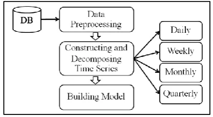
In this research, our main objective was to find a model to efficiently forecast the electricity consumption in a household by applying Box and Jenkins method. The suitable forecasting methods were chosen for finding the method that was suitable for short term analysis in daily, weekly, monthly, and quarterly. The proposed forecasting time series process and the steps are shown in Fig.1.

Fig. 1. The framework of steps for building the forecasting time series models.

From Fig. 1, we can explain in detail of each step as follows.

A. Data Preprocessing

This research used data set [14] about electric power consumption in one household that has a sampling rate in one minute over a long period of time from the years 2006 to 2010. We used R and Rstudio for building the model. The first step is to read the text file (as show in Fig. 2) with the following R commands:

hPower<-read.table("household_power_consumption.txt" , header=T, sep=";")

tmp_hPower<-hPower[,1:3]

#Used date, time and global_active_power only.

Fig. 2. Example of data recording electric power consumption in household.

The raw data are not ready for constructing forecasting model because some values are missing and the recorded time frames are inappropriate. We have to do the following preprocessing task.

1. Fill the missing data.

The lack of some information may decrease the predictive efficiency of the forecasting model. The methods for fill missing data are varied such as fill with mean, median or previous value. In this research, we used the previous value for missing value imputation with the assumption that the current data will be similar to the previous ones. The steps for filling missing data using the R commands are shown below and the result can be displayed in Fig. 3.

library(“zoo”)

NAs <- tmp_hPower == "?" is.na(tmp_hPower)[NAs] <- TRUE tmp_hPower$Global_active_power <-

na.locf(tmp_hPower$Global_active_power, fromLast = FALSE) # na.loc is command to fill missing value.

Fig. 3. Fill the missing data with the previous value “0.244”. 2. Change the data format.

The dataset are in the unit of a minute. So, we used the aggregate function in R to format data to suit the forecasted period. For example, aggregate data to be monthly can be performed with the following code and the result is show in Fig.4.

agg_Month

<-aggregate(trainData,by=list(as.yearmon(trainData$hP_Date,"%d %m%Y")), FUN=mean, na.rm=TRUE)

B. Constructing and decomposing time series format This step uses the data series that are in the appropriate format for time series construction and decomposition with the following two steps:

1. Time series construction

We used the ts() function in R library for construction of a time series. This function must be specifying a frequency of time series. This paper used a frequency of 365, 53, 12, and 4 to indicate that a time series is composed of daily series, weekly series, monthly series, and quarterly series, respectively. We set the parameters frequency= 53 and start = c(2006,51) for weekly series starting from week 51 of the year 2006.

tsWeek <-ts(hPower_ByWeek[,2],frequency=53,start=c(2006,51))

2. Time series decomposition

This step is to decompose a time series into trend, seasonal, cyclical and irregular components, by applying the decomposed() function as below:

fW <-decompose(tsWeek)

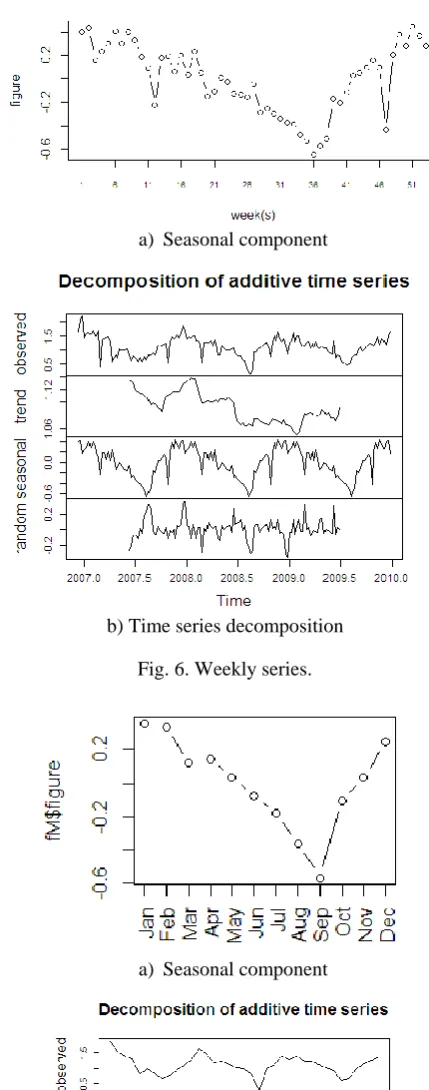
The seasonal of time series from a smaller unit of daily to a large unit of quarterly are shown in Fig.5 (a) to 8(a), and time series decomposition are shown in Fig.5 (b) to 8(b).

a) Seasonal component

b) Time series decomposition Fig. 5. Daily series.

a) Seasonal component

b) Time series decomposition Fig. 6. Weekly series.

a) Seasonal component

a) Seasonal component

b) Time series decomposition Fig. 8. Quarterly series.

From Fig.5 (b) to 8(b), the chart in a top level is the original time series. The chart below the top one is trend in time series, and below the trend chart showing seasonal factors. The chart at the bottom of the figure is the remaining part after removed trend and seasonal components.

C. Building Models

The forecasting method that we used in this research is the Box and Jenkins method to build the ARIMA and ARMA models.

1. ARIMA : Autoregressive Integrated Moving Average The steps for constructing ARIMA model and forecasting time series are as follows:

Step 1: Determine the suitable order for ARIMA(p,d,q), which can be considered from ACF (Autocorrelation function) and PACF (Partial autocorrelation function). In R language, there is a function to find order (p,d,q) automatically, and can be shown as follows:

install.package(“forecast”) library(“forecast”)

auto.arima(x) # x is time series data

Orders that are suitable for daily, weekly, monthly, and quarterly series are ARIMA(3,1,3), ARIMA(1,0,1), ARIMA(0,0,0) and ARIMA(0,0,0), respectively.

Step 2: The appropriate order was used for constructing model and forecasting time series. For example, in weekly series, the R commands are as the following and the running result was shown in Fig. 9.

# ARIMA model

fitWeek <- arima(tsWeek, order=c(1,0,1) ,list(order=c(0,1,0), period=53))

# Forecasting 48 weeks with test dataset.

foreWTest <- predict(fitWeek,newdata=testData_ByWeek, n.ahead=48)

Fig. 9. Weekly Times series forecasting.

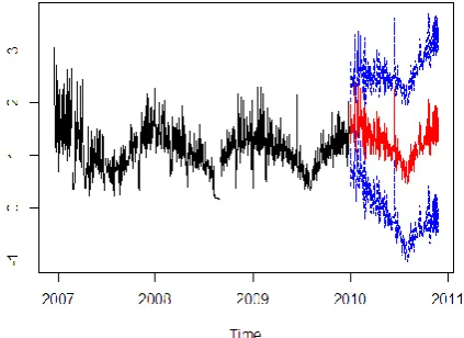
Then, the time periods of forecasting in daily, monthly, and quarterly series are set to be 330, 11, and 4, respectively. The results were illustrated in Fig. 10 to 12.

Fig. 10. Daily Times series forecasting.

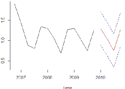
Fig. 12. Quarterly Times series forecasting. From Figs.9 to 12, the black lines from years 2006 to 2010 show the actual data, whereas the red lines (the middle trend line from the year 2010 to 2011) show the forecasted value and the two dotted lines above and below the red line 3 are error bounds at confidence levels 95%.

2. ARMA : Autoregressive Moving Average

The appropriate order from step 1 of ARIMA model construction was used for constructing the ARMA(p,q) model and forecasting time series. The R commands for constructing ARMA model in a weekly series are as follows:

install.packages("fArma") library(fArma)

# ARMA model

fitWeek_ARMA <- armaFit(~arma(1,1), data = tsWeek) # Forecasting 10 weeks with test dataset.

predict(fitWeek_ARMA, newdata = testData_ByWeek,n.ahead=10, n.back = 8, conf = c(80, 95),doplot = TRUE)

Fig. 13. Weekly Times series forecasting model. Running result of a weekly model is shown in Fig.13. Then, the time period for forecasting in daily, monthly and quarterly series are set to be 10, 20, 20 and their running results are shown in Figs. 14 to 16, respectively.

Fig. 14. Daily Times series forecasting model.

Fig. 15. Monthly Times series forecasting model.

Fig. 16 Quarterly Times series forecasting model

IV. EXPERIMENTAL EVALUATION

This research used electric consumption in one household dataset obtained from UCI Machine Learning Repository [14] for evaluating the time series models. This dataset has 9 attributes and 2,075,259 transactions. The time series data was divided into two groups. The first group was training dataset which contain data from 2006-12-26 to 2009-12-31 for construction the forecasting models. The second group was test dataset which contain data from 2010-01-01 to 2010-11-26 for finding the most suitable forecasting period.

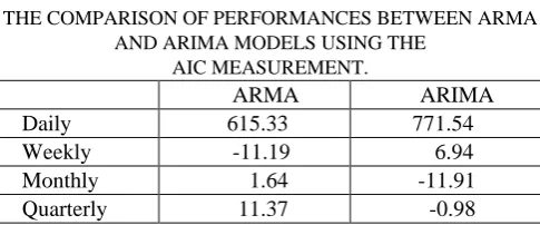
(Akaike Information Criterion), was summarized in Table 1. The lower the AIC value, the better the model.

TABLE I

THE COMPARISON OF PERFORMANCES BETWEEN ARMA AND ARIMA MODELS USING THE

AIC MEASUREMENT.

ARMA ARIMA

Daily 615.33 771.54 Weekly -11.19 6.94 Monthly 1.64 -11.91 Quarterly 11.37 -0.98 From Table 1, we can see that the ARIMA model can represent monthly and quarterly series, whereas the ARMA model can represent daily and weekly series. Then, the time horizon of forecasting were calculated and short terms forecasting were chosen by considering the smallest value of Root Mean Square Error (RMSE). Forecasting results are summarized in Table 2.

TABLE II

THE COMPARISON OF FORECASTING PERFORMANCE EVALUATED BY RMSE

Forecast RMSE

ARMA Daily 7 0.34

14 0.35

21 0.32

28 0.29

35 0.32

42 0.36

Weekly 1 0.30

5 0.18

10 0.20

15 0.18

20 0.18

25 0.18

30 0.24

ARIMA Monthly 2 0.10

4 0.10

6 0.09

8 0.09

10 0.09

Quarterly 1 0.03

2 0.02

3 0.38

4 0.05

From Table 2, the time forecasting shows the lowest RSME for daily series as 28 days at 0.29. The next best forecasting unit is 35 days at error rate 0.32. For weekly series of 5, 15, 20 and 25 weeks have equal error rate at 0.18, followed by 10 weeks at 0.20, for monthly series as 6, 8 and 10 months at 0.09, followed by 2 and 4 at 0.10, and quarterly series as 2 quarters at 0.02, followed by 1 at 0.03 and 4 at 0.05.

V. CONCLUSIONS

The purpose of this research was to find a suitable model to forecast the electric consumption in a household, and to find the most suitable forecasting period (in daily, weekly, monthly, or quarterly). We used the ARIMA and ARMA models for forecasting the individual household electric power consumption from December 2006 to November 2010. Then, chose the suitable forecasting method and identified the most suitable forecasting period by considering the smallest values of AIC and RMSE, respectively. The results showed that the ARIMA model can represent the most suitable forecasting periods in monthly and quarterly. On the other hand, ARMA model can represent the most suitable forecasting periods in daily and weekly. Then, we calculated the most suitable forecasting periods and it showed that the method were suitable for short term periods ranging from 28 days, 5 weeks, 6 months to 2 quarters.

REFERENCES

[1] Bruce L. Bowerman, Richard T. O’ Connell, & Anne B. Koehler, “Forecasting, time series, and regression: an applied approach,” 4th ed. The United States of America: Thomson Brooks, 2005.

[2] Makridakis, S., S.C. Wheelwright and R.J. Hyndman, “Forecasting: Methods and Applications,” 3 ed. Wiley, Inc., New York, 1998. [3] Box, G.E.P. and G. Jenkins, “Times Series Analysis Forecasting and

Control,” Holden-Day, San Francisco, CA, 1976. [4] [Online]. Available: http://www.rstudio.com/ [5] [Online]. Available: http://cran.us.r-project.org/

[6] Jonathan D. Cryer & Kung-Sik Chan, “Time series analysis: with applications in R,” 2nd _{ed. New York: Springer, 2008.}

[7] Robert H. Shumway & David S. Stoffer, “Time Series Analysis and Its Applications with R Examples,” 3rd _{ed. New York: Springer, 2011.}

[8] Oleg Nenadic, Walter Zucchini, “Statistical Analysis with R - a quick start -,” Retrieved November 10, 2012, from

http://www.scribd.com/doc/114263559/Statistical-Analysis-With-R-A-Quick-Start.

[9] Samer Saab, Elie Badr and George Nasr, “Univariate modeling and forecasting of energy consumption: the case of electricity in Lebanon,” Energy, vol.26, 2001, pp. 1-14.

[10] Qing Zhu, Yujing Guo, Genfu Feng, “Household energy consumption in China forecasting with BVAR model up to 2015,” 2012 Fifth International Joint Conference on Computational Sciences and Optimization, 2012.

[11] Volkan Ş. Ediger, Sertaç Akar, “ARIMA forecasting of primary energy demand by fuel in Turkey,” Energy Policy, vol.35, 2007, pp. 1701-1708.

[12] Javier Contreras, Rosario Espinola, Francisco J. Nogales, and Antonio J. Conejo, “ARIMA models to predict next-day electricity prices. Power Systems,” IEEE Transactions on 2003, vol.18, no. 3, pp. 1014-1020.

[13] Antonio J. Conejo, Miguel A. Plazas, Rosa Espinola, and Ana B. Molina, “Day-ahead electricity price forecasting using the wavelet transform and ARIMA models,” IEEE Trans. Power Syst., vol. 20, no. 2, 2005, pp. 1035–1042.