NUCLEAR MAGNETIC RESONANCE SPECTROSCOPY AND COMPUTATIONAL METHODS FOR THE CHARACTERIZATION OF
MATERIALS IN SOLUTION AND THE SOLID STATE
Diego Carnevale
A Thesis Submitted for the Degree of PhD at the
University of St. Andrews
2010
Full metadata for this item is available in Research@StAndrews:FullText
at:
https://research-repository.st-andrews.ac.uk/
Please use this identifier to cite or link to this item: http://hdl.handle.net/10023/1349
This item is protected by original copyright
Nuclear Magnetic Resonance spectroscopy
and computational methods
for the characterization of materials
in solution and the solid state
A Thesis submitted for the degree of
Doctor of Philosophy
in the
School of Chemistry
University of St Andrews
by
Diego Carnevale
I, Diego Carnevale, hereby certify that this thesis, which is approximately 50000 words in length, has been written by me, that it is the record of work carried out by me and that it has not been submitted in any previous application for a higher degree.
I was admitted as a research student in September 2006 and as a candidate for the degree of PhD in September 2006; the higher study for which this is a record was carried out in the University of St Andrews between 2006 and 2010.
Date Signature of candidate
I hereby certify that the candidate has fulfilled the conditions of the Resolution and Regulations appropriate for the degree of PhD in the University of St Andrews and that the candidate is qualified to submit this thesis in application for that degree.
In submitting this thesis to the University of St Andrews I understand that I am giving permission for it to be made available for use in accordance with the regulations of the University Library for the time being in force, subject to any copyright vested in the work not being affected thereby. I also understand that the title and the abstract will be published, and that a copy of the work may be made and supplied to any bona fide library or research worker, that my thesis will be electronically accessible for personal or research use unless exempt by award of an embargo as requested below, and that the library has the right to migrate my thesis into new electronic forms as required to ensure continued access to the thesis. I have obtained any thirdparty copyright permissions that may be required in order to allow such access and migration, or have requested the appropriate embargo below.
The following is an agreed request by candidate and supervisor regarding the electronic publication of this thesis:
Access to printed copy and electronic publication of thesis through the University of St Andrews.
Date Signature of candidate
Contents
Contents I
Abstract VII
Acknowledgements VIII
1 Introduction 1
1.1 Thesis overview 1
1.2 Experimental and computational details 3
1.2.1 Solution-phase NMR 3
1.2.2 Solid-state NMR 4 1.2.3 Calculations 5
2 Quantum mechanical description of NMR 7 2.1 Spin operators 7 2.2 The superposition state 8 2.3 Bulk magnetization 9
2.4 Density operator 10
2.5 Coherences 11
2.6 Time evolution of the density operator 12
2.7 Rotations 13
2.8 Hamiltonians 14
2.9 Average Hamiltonian Theory 16
2.10 The magnetic field 19
2.11 Pulses 20
2.12 The chemical shielding 23
2.13 Multispin systems 26
2.14 The dipolar coupling 27
2.15 J coupling 29
2.17 Detection 32
2.18 Solution-phase NMR 33
2.19 Spin echoes 35
3 Basic techniques in NMR 37
3.1 Fourier transform 37
3.2 2D NMR 39
3.2.1 Phase-modulated 2D data set 39
3.2.2 Amplitude-modulated 2D data set 41
3.3 Phase cycling 43
3.3.1 Nested phase cycling 43
3.3.2 Cogwheel phase cycling 45
3.4 Pulse field gradients 45
3.5 Magic-angle spinning 47
3.6 Spinning sidebands 50
3.7 Heteronuclear decoupling 52
3.7.1 TPPM 53
3.7.2 SPINAL 54
3.8 Homonuclear decoupling 54
3.8.1 Lee-Goldburg decoupling 55
3.9 Cross polarization 56
3.10 INEPT 58
4 Density functional theory for the calculation
of NMR parameters 61
4.1 DFT concepts 61
4.2 Basis sets 64
4.2.1 Atomic orbitals 65
4.2.2 Planewaves 67
4.3.1 GIAO 71
4.3.2 CSGT 71
4.3.3 GIPAW 72 5 Solution-phase NMR and DFT characterization of chiral fluoropolymer 73
5.1 Introduction 73
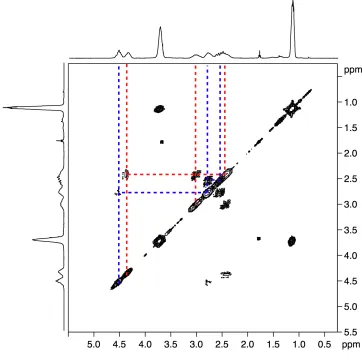
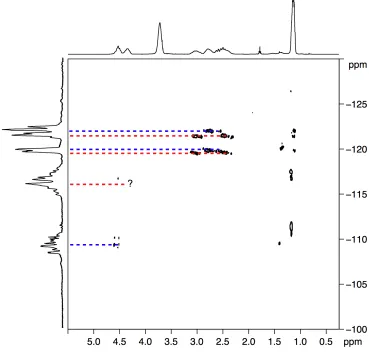
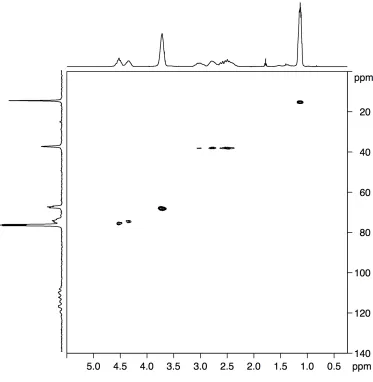
5.2 Additional NMR methodologies 75 5.2.1 Heteronuclear Multiple Quantum Correlation 75 5.2.2 Heteronuclear Single Quantum Correlation 77
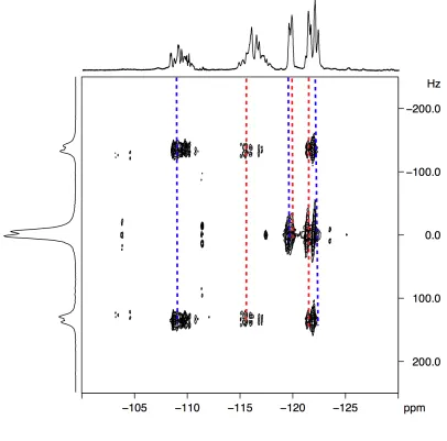
5.2.3 Homonuclear J-resolved spectroscopy 78 5.3 Stereochemistry of PCCE 79 5.4 1H NMR data analysis 80 5.5 13C NMR data analysis 81 5.6 19F NMR data analysis 82 5.7 Heteronuclear-correlation and homonuclear J-resolved analysis 84 5.8 Computational study 91
5.9 Analysis of 19F computational results 94 5.10 Analysis of 1H computational results 96 5.11 Analysis of 13C computational results 97 5.12 Conclusions 98
6 14/15N solution-phase NMR and DFT calculations of organic templates for solid-state synthesis 100
6.1 Introduction 100
6.2 DFT modeling of BDAB 102
6.3 Solution-phase NMR study of BDAB 105
6.4 Analysis of experimental and calculated data 111
7 NMR and DFT studies of boroxoaromatic systems
in the solid state 114
7.1 Introduction 114
7.2 Additional NMR methodologies 116
7.2.1 Heteronuclear Multiple Bond Correlation 116
7.2.2 Dipolar dephasing 118
7.2.3 HETCOR 120
7.2.4 MQMAS 121
7.3 Results and discussion 123
7.3.1 HBOP solution-phase NMR 124
7.3.2 BBE solution-phase NMR 129
7.3.3 HBOP DFT calculations in the vacuum 133 7.3.4 BBE DFT calculations in the vacuum 139
7.3.5 HBOP solid-state NMR 144
7.3.6 Solid-state DFT calculations of HBOP 149
7.3.7 BBE solid-state NMR 154
7.3.8 Solid-state DFT calculations of BBE 160
7.3.9 Solid-state reaction 165
7.3.10 Semiempirical calculations of the
mechanism of reaction 167
7.4 Conclusions 169
8 Measurement of chemical shift anisotropy
in the solid state 171
8.1 Introduction 171
8.2 CSA amplification 172
8.3 CSA amplification in AHT 175
8.4 CSA Amplification and CSA-Amplified PASS
8.5 Results 178
8.5.1 Amplification factor 180
8.5.2 Pulse miscalibration 184
8.5.3 Transmitter offset 188
8.6 The effect of the homonuclear dipolar interaction 192
8.7 119Sn and 89Y CSA amplification 197
8.8 Conclusions 202
9 CP and nutation processes of quadrupolar nuclei
under static and MAS conditions 204
9.1 Introduction 204
9.2 Theory of quadrupolar CP 206
9.3 Theory of quadrupolar nutation 209
9.4 Results 211
9.4.1 Simulations of static CP
and nutation spectra 211
9.4.2 CP and nutation under MAS 224
9.5 Comparison between static-
and spinning-system results 235
9.6 Influence of contact time,
dipolar interaction and spinning rate 238 9.7 Spin-locking efficiency and
rotor-driven interconversion of coherences 241
9.8 Conclusions 246
10 General conclusions 247
Appendix A 251
Appendix B 252
Appendix D 256
Appendix E 258
Appendix F 268
Abstract
Acknowledgements
I am extremely thankful to my supervisor, Dr Sharon E. Ashbrook, for giving me the possibility to join her research group, her restless assistance, advice and support. I am grateful to the EPSRC for funding the work hereby presented.
I must also thank Professor Steve Wimperis, Dr Melinda Duer, Dr Steven Brown and Dr Stefan Steuernagel for experimental time and advice. I am very thankful to Dr Philip Wormald, Dr Paul Wright and Professor Douglas Philp for the work done in collaboration with them. My gratitude also goes to Dr Tomas Lebl and Melanja Smith for assistance in the solution-phase experiments and to Dr Herbert Fruchtl, Dr Tanja Van Mourik and Professor Chris Pickard for help and advice in the computational work. A special thanks must also go to Dr Robin Orr for the invaluable help in setting up his experiment and the numerical simulations widely utilized in this work.
I thank all the members of the Ashbrook group I had the special pleasure to meet in these years. In particular, Dr John Griffin, Karen Johnston, Martin Mitchell, Valerie Seymour and Daniel Dawson.
Chapter 1
Introduction
1.1 Thesis overview
NMR spectroscopy1, 2 is perhaps the most valuable tool for the structural investigation of chemically relevant systems. The high resolution easily achievable in the solution phase3 allows the characterization of very large systems such as biological macromolecules, probing their interactions with the environment and their dynamic processes upon which life is based. The anisotropic nature of the physical interactions in the solid state4 on the other hand, significantly compromises the resolution of the NMR technique. Nevertheless, precious insights into the local chemical environment of materials can be obtained by exploiting the anisotropic interactions themselves. Furthermore, recent improvements in hardware5-7 and the development of new and complex pulse sequences have advanced solid-state NMR to the point where it is now an indispensable probe of structure, order and dynamics in the solid state.8
The actual use of spectrometers relies upon a variety of experimental techniques which allow scientists to efficiently detect and process NMR signals. In Chapter 3, an overview of the most well-established NMR experimental methodologies is reported. These cover procedures for data processing, selection of desired coherences, acquisition of high-resolution spectra and detection of low-abundant and low-! nuclei.
Computational methods increasingly play an important role in scientific research since they provide a means of supporting experimental results on a theoretical basis. In chemistry, the computational estimation of the properties of materials is a powerful tool for driving the rational designing of new systems. From the NMR point of view, the capability to compute key parameters such as chemical shielding, J couplings or electric field gradients can prove to be indispensable a tool for structural characterization, spectral interpretation and assignment. In the past decades, density functional theory (DFT) has proven to be perhaps the most robust and less time-demanding method to approach the study of most chemical systems and their relevant properties. Chapter 4 presents an introduction to the DFT methods used in this thesis and the relevant NMR parameters that can be computed.
In Chapter 5, the characterization of a polymer obtained from the polymerization of a chiral fluorinated building block is reported. The study is based upon a combination of solution-phase NMR techniques and DFT calculations. The analysis of the stereochemical variety of the system is approached with an original computational scheme and the definition of a stereochemically-related shielding parameter that helps to rationalize the experimental 19F spectral complexities. The sample was obtained from Dr Philip Wormald from the School of Chemistry, University of St Andrews.
In Chapter 7 a combination of solution- and solid-state NMR, supported by DFT calculations is reported for the structural characterization of the covalent self-assembly boroxophenanthrene/bis-(boroxophenanthryl)ether system in both the solution and solid state. The solid-state reactivity of these two related compounds is also investigated. A semiempirical computational approach is employed to obtain insight into the mechanism of interconversion between the two compounds. All samples were obtained from Professor Douglas Philp and Dr Vicente del Amo from the School of Chemistry, University of St Andrews.
In the study reported in Chapter 8, two NMR methods for the measurement of chemical shift anisotropy (CSA) in the solid state are analyzed and tested using simple 13C and 31P containing model compounds. The influence of homonuclear dipolar interactions on the accuracy of the measurements is investigated with numerical calculations. Extension of the available methods to the more challenging investigation of 119S and 89Y containing materials is also reported.
In the work reported in Chapter 9 previous studies concerning cross polarization (CP) and nutation experiments for quadrupolar nuclei in the solid state under static conditions are corroborated with a more detailed computational model and extended to include the effects of magic-angle spinning (MAS). Simulations for both single- and multiple-quantum CP and nutation processes are investigated for a I = 3/2 23Na nucleus.
1.2 Experimental and computational details
1.2.1 Solution-phase NMR
NMR tubes. All spectra were acquired at 25 °C and all the pulse sequences utilized employed PFG for coherence selection. All 1H 1D spectra were recorded using a pulse of flip-angle of 30° (! 4 µs) and recycle interval of 1 s. A line broadening of 0.3 Hz was applied in most cases. All 13C 1D spectra were recorded using a pulse of flip-angle of 30° (! 4 µs) and recycle interval of 2 s. A line broadening of 2 Hz was applied prior to FT unless stated. All 19F 1D spectra were recorded using a pulse of flip-angle of 30° (! 3 µs) and recycle interval of 1 s. A line broadening of 0.3 Hz was applied to the signal. 1H and 19F COSY spectra were processed with a sine-bell weighting function applied to both dimensions. All 1H-13C HSQC 2D spectra utilized 3.45 ms coherence transfer period for the selection of 1J heteronuclear correlations of 140 Hz and a 90° shifted squared sine-bell weighting function was applied in both dimensions. All 1H-13C HMBC 2D spectra utilized 62.5 ms coherence transfer period for the selection of 1J heteronuclear correlations of 8 Hz and a sine-bell weighting function was applied in both dimensions. The 1H-19F HMQC 2D spectra utilized 55.6 ms coherence transfer period for the selection of 1J heteronuclear correlations of 9 Hz and a 45° shifted squared sine-bell weighting function was applied in both dimensions. The 19F J-resolved 2D spectrum was processed with a sine-bell window function in both dimensions. All 2D spectra were performed using 256 increments in the indirect dimension with the exception of the 19F J-resolved spectrum for which 128 increments were used. All the 90 and 180° pulses are related to the 30° values previously mentioned.
1.2.2 Solid-state NMR
BPO4 (11B –3.3 ppm, 31P –29.5 ppm) Y2Ti2O7 (89Y 65.0 ppm) and SnO2 (119Sn –604.3 ppm). Typical 90° pulse lengths were usually 2.5 or 3 µs corresponding to rf field strengths between 80 and 100 kHz. 13C spectra were acquired using cross-polarization with a ramped (90-100%) spin-lock pulse on 1H and a contact time of 2 ms. Recycle intervals between 1 and 70 s were used as required. Either TPPM or SPINAL32/64 heteronuclear decoupling were employed during acquisition. FSLG homonuclear decoupling was employed in the indirect dimension of the 1H-13C HETCOR experiment and magnetization transfer was achieved with a 0.1 ms contact time in the CP step. Quadrature detection in the indirect dimension was achieved using States-TPPI. 11B spectra were acquired using a CT selective spin-echo pulse sequence to minimize the background contributions from the probe. MQMAS experiments were performed using a phase-modulated split-t1 shifted-echo pulse sequence with heteronuclear CW 1H decoupling. In some cases, a line broadening weighting function was utilized for the processing of the raw data. CSA amplification experiments were performed using the pulse sequences discussed in Chapter 8. Cogwheel phase cycling was used in all the CSA-Amplified PASS experiments and in some CSA Amplification experiments. Conventional nested phase cycling was employed in all the other cases. Further experimental details for specific spectra can be found in figure captions.
1.2.3 Computational details
Table 1.1 Basis sets used for convergence of the calculated isotropic shieldings using Gaussian03 and related indexes utilized in the studies presented in this thesis. The first four basis sets are double-zeta split valence whereas the second four are triple-zeta split valence basis sets.
Basis set Index
6-31G(d,p) 1
6-31+G(d,p) 2
6-31++G(d,p) 3
6-31++G(2d,p) 4
6-311G(d,p) 5
6-311+G(d,p) 6
6-311++G(d,p) 7
6-311++G(2d,p) 8
DFT calculations for solid-state systems were carried out using CASTEP10 (version 4.3), a planewave pseudopotential code which exploits the inherent periodicity associated with many solids. The GGA PBE functional and the GIPAW algorithm were used for the calculation of the NMR parameters. Geometry optimization was performed when necessary within CASTEP with the same functional. Typical k-point spacing and cut-off energies of 0.05 Å–1 and 700 eV, respectively, were used. All calculations were performed on up to four four-processor nodes of the EaStCHEM Research Computing Facility.
Semiempirical calculations were carried out using the PM6 method11 as implemented in the MOPAC200912 code. Reaction coordinates were driven using the POINT and STEP keywords and the step size was set to 0.05 Å in all cases. All calculations were performed on a 8-processor local cluster.
Chapter 2
Quantum mechanical description of NMR
2.1 Spin operators
The spin state of a nucleus is described by a nuclear spin wavefunction !spin. In order to determine the spin properties of the nuclear system, spin operators which act on !spin are required. These are the operator defining the magnitude of the nuclear spin squared Iˆ2and its components Iˆx, Iˆy and Iˆz.
16 The relation between them is expressed by:
ˆ I2 = ˆ
Ix+Iˆy+Iˆz. (2.1)
ˆ
I2 and ˆ
Iz commute (i.e., [Iˆ 2
, ˆIz] = 0) therefore they have the same eigenfunctions I,m . These are specified by the spin quantum number I (0,1/2, 1, 3/2…) and the azimuthal quantum number m (!I...+I). Disregarding for simplicity the factor ! in the eigenvalues:
ˆ I2
I,m =I I
(
+1)
I,m (2.2)ˆ
Iz I,m =m I,m . (2.3)
The corresponding expectation values17 are:
ˆ
I2 = I,m Iˆ 2
I,m
I,m I,m =I I
(
+1)
(2.4)ˆ
Iz =m. (2.5)
For a nucleus with spin quantum number I=1/2, the two states 1 / 2,+1 / 2 and
I2 = 3 4 1 0 0 1 ! "# $ %& ; Iz =
1 2 1 0 0 !1 " #$ % &' (2.6)
Ix = 1 2 0 1 1 0 ! "# $
%& ; Iy=! i 2 0 1 !1 0 " #$ %
&'. (2.7)
It is also convenient to define raising and lowering operators Iˆ+and Iˆ! given by:
I+ = 0 1
0 0 ! "#
$
%& ; I! = 0 0 1 0 " #$
%
&'. (2.8)
The relations between Iˆx and Iˆy and the raising and lowering operators are:
ˆ Ix = 1
2 ˆ I++Iˆ!
(
)
; Iˆy = 1 2iˆ I+!Iˆ!
(
)
. (2.9)Both the x- and y-components of the angular momentum operator are therefore expressible as linear combinations of the lowering and raising operators.
2.2 The superposition state
The actual spin state of a nuclear system is fully described by a superposition of its available states. This is expressed by a linear combination of the 2I+1
eigenfunctions.19 For a spin I = 1/2 nucleus, therefore:
! = cm I,m m="I
I
#
=c$ $ +c% % . (2.10)Since Iˆ
x, Iˆy and Iˆz do not commute with each other (i.e., [Iˆx, ˆIy] = iIˆz and the
respective cyclic permutations), ! and ! are not eigenfunctions of Iˆ
xand Iˆy.
However, it can be shown that:
ˆ Ix ! =
1 2 " ;
ˆ Ix ! =
1
2 " (2.11)
ˆ
Iy ! =
1 2i " ;
ˆ
Iy ! ="
1
2i# . (2.12)
Their expectation values are:
ˆ
Ix =
! Ix !
! ! =
1 2c"
#c
$+1
2c$ #c
" (2.13)
ˆ
Iy =
i 2c!
"c #$ i
2c#
"c
Equations (2.13) and (2.14) show that the expectation values of Iˆx and Iˆy depend
only on the coefficients weighting the available states for the spin as expressed in its
superposition-state description.18
2.3 Bulk magnetization
The oscillating voltage which is detected in an NMR experiment arises from the bulk
magnetization Mz generated within the sample when an external magnetic field is
applied (along the z-axis by convention). This magnetization is the vectorial sum of
all the magnetic moments µz of the nuclear spins present in the sample:
Mz = µz,i i=1
N
!
. (2.15)The magnetic moment µz is related to the expectation value of the spin operator Iˆ z
via the gyromagnetic constant ! and its ensemble average is given by:
µz =! Iˆ
z =! pi i=1
N
"
#i Iˆz #i , (2.16)where pi is the probability of the i-th spin being in the spin state !i . Therefore the
bulk magnetization and its x and y components can be expressed as:
Mz =
1 2!N c"
#c
" $c%#c%
(
)
(2.17)Mx= 1 2!N c"
#
c$+c$#c"
(
)
(2.18)My= i
2!N c" #c
$ %c$#c"
(
)
. (2.19)2.4 Density Operator
Given the dependence of the magnetization on the coefficients c! and c! only, a
more convenient approach to describe the spin state of a multi-spin system can be
achieved through the definition of an operator directly expressible through these
coefficients only. As already shown in Equation 2.16, the expectation value of a
generic operator Aˆ over an ensemble average can be written as:
ˆ
A = pi i
!
"i Aˆ "i . (2.20)Expressing the i-th wavefunction in a generic superposition state of !i,j basis set
functions so that !i = ci,j
j
"
#i,j and !i = ci,j"
j
#
$i,j , Equation (2.20) becomes:ˆ
A = pi
i
!
ci,j"
j
!
#i,j Aˆ ci,j j!
#i,jˆ
A = pi i,j
!
ci,jci,j " #i,j Aˆ #i,j . (2.21)
Introducing a new operator !ˆ = pi
i,j
"
ci,jci,j# referred to as density operator,16 Equation
(2.21) is more compactly rewritten as:
ˆ
A =! "ˆ i,j Aˆ "i,j
ˆ
A = !i,j "ˆAˆ !i,j =Tr#$ %&"ˆAˆ . (2.22)
The remarkable property of the density operator stems from the fact that any property
related to the operator Aˆ of an ensemble average system of n spins can be computed
from the density operator without the need to compute the eigenvalues of Aˆ n times
for each spin. The matrix representation of !ˆ with elements !ij = i !ˆ j is:
!= !11 !12
!21 !22
" #$
% &' =
c()c( c()c*
c*)c( c*)c*
" # $ $ % & '
' . (2.23)
The bulk magnetization components in the density operator formalism then become:
Mz = 1
Mx=
1
2!N
(
"21+"12)
(2.25)My= i
2!N
(
"12 #"21)
. (2.26)Equations (2.24), (2.25) and (2.26) show that all the components of the bulk magnetization are, coherently with Equations (2.17), (2.18) and (2.19), expressible in terms of density matrix elements.
2.5 Coherences
The diagonal elements of the density matrix are referred to as populations of the !
and ! states. The off-diagonal elements are referred to as coherences19 between the
! and ! states. Expressing the complex coefficients in terms of a real magnitude
ai and a phase !i yields:
c! =a!exp
{
i"!}
; c!" =a!exp{
#i$!} (2.27)c! =a!exp
{
i"!}
; c!" =a!exp{
#i$!}
. (2.28)The density matrix becomes:
!= a"2 a"a#e
i($"%$#) a#a"e%i($"%$#)
a#2
&
' ( (
)
* +
+. (2.29)
When the phases !i of the ensemble average are randomly distributed, the
off-diagonal elements average to zero due to destructive interference of the
exp
{
±i(
!"#!$)}
phase factors. These off-diagonal elements are non-zero only ifthere is phase coherence between the ! and ! states and are therefore referred to
as coherences. Coherences are classified according to their order p. For a !rs
coherence, its prs order is defined as the difference between the azimuthal quantum
numbers related to the r and s states:
prs =mr!ms
prs =
I,r Iˆz I,r
I,r I,r !
I,s Iˆz I,s
For an ensemble averaged of non-interacting nuclei with spin quantum number
I =1/2 there can only be ±1 coherence orders (single-quantum (SQ) coherences).
Higher order coherences (multiple-quantum (MQ) coherences) can be associated with
either a quadrupolar spin (I >1 / 2) or with a system of multiple interacting spins, for
which the density matrix is obtained by direct product of the single-spin density
matrices. Therefore the detection of MQ coherences in a I =1/2 spin system indicates
interaction between single spins.
2.6 Time evolution of the density operator
Considering the time-dependent Schrödinger equation d ! /dt ="iHˆ ! , its
complex conjugate d ! /dt =iHˆ ! and the partial derivative of the ! !
product wavefunction:
! " " !t =
!" !t " +
! "
!t " =#i
ˆ
H," "
$% &'. (2.31)
The ensemble average of Equation (2.31) describes the time evolution of the density
operator:20
d!ˆ
( )
t dt ="iˆ
H, ˆ!
( )
t#$ %&. (2.32)
Equation (2.32) is referred to as the Liouville-von Neumann equation and has the
general solution:21
ˆ
!
( )
t =U tˆ( )
!ˆ( )
0 Uˆ"1( )
t . (2.33)The U tˆ
( )
operator is termed propagator as it propagates the initial density operatorˆ
!
( )
0 to that which describes the system at time t. The propagator, via theHamiltonian, carries the information regarding the all interactions to which !ˆ
( )
0 issubject between t=0 and t. If the Hamiltonian is time independent, the propagator
takes the simpler form:
ˆ
U t
( )
=exp{ }
!iHtˆ . (2.34)If the Hamiltonian is time dependent but commutes with itself at different times
ˆ
U t
( )
=exp !i H tˆ( )
0 t
"
dt # $ % & '(. (2.35)
If the Hamiltonian is time dependent and does not commute with itself at different
times, the propagator is expressed by:
ˆ
U t
( )
=Tˆexp !i H tˆ( )
0 t
"
dt # $ % & '(. (2.36)
The Dyson time-ordering operator Tˆ,22 needed when non-commuting time-dependent
Hamiltonians are involved, ensures the terms of the product are evaluated in strictly
chronological order. For the latter two cases of time-dependent Hamiltonian, the
propagator can be numerically approximated by:
ˆ
U t
( )
=lim!t"0 exp i ˆ
H n
( )
!t !t{
}
n=0
t/!t
#
. (2.37)It is this latter formulation which is used for the numerical evaluation of the time evolution of density matrix elements (i.e., coherences) in the simulations of NMR experiments.
2.7 Rotations
It is often useful in the quantum-mechanical description of NMR phenomena to rotate
objects such as wavefunctions or operators (active rotations). Rotations are achieved
with rotation operators16 Rˆ
! =exp
{
"i#Lˆ!}
where Lˆ! is the operator for the ! component of the angular momentum defined as:ˆ L!=1
i ˆ " #
#$ %$ˆ # #" & ' ( ) *
+, (2.38)
where !ˆ and !ˆ are the operators for position along the " and # axes respectively. Rˆ ! acts on the object so as to rotate it about the ! axis by an angle $. A general
wavefunction ! is transformed by Rˆ! to produce !R so that !R =Rˆ" ! or
! =Rˆ
"#1 !R =exp
{ }
i$Lˆ" !R . It can be proven that a series expansion ofexp
{
!i"Lˆ#}
$ˆ=$ˆcos( )
" +%ˆsin( )
" =$ˆR. (2.39)The rotation operator Rˆ
! can also be used to rotate other operators according to the
expression Oˆ
R =Rˆ!OˆRˆ!
"1 or Oˆ =Rˆ
!"1OˆRRˆ!. Considering the general operators Aˆ, Bˆ
and Cˆ, if their cyclic permutations of commutators [A, ˆˆ B] = iCˆ apply, the following transformation exists:
exp
{ }
!i"Aˆ Bˆexp{ }
i"Aˆ =Bˆcos( )
" +Cˆsin( )
" . (2.40)Rather than rotate an object (wavefunction or operator), it is equivalently possible to
rotate the frame of reference in which that object is expressed. The relationship
between the wavefunction ! expressed in the old frame and !R expressed in the
new frame is !R =Rˆ"
#1 ! or ! = ˆ
R" !R . Similarly, for a general operator Oˆ in
the old frame, OˆR =Rˆ!"1OˆRˆ! or Oˆ =Rˆ!OˆRRˆ!"1. Comparing active and passive rotations
the rotation operator Rˆ! is replaced by its inverse Rˆ!"1. This is because to rotate an
object by an angle ! around the " axis is equivalent to rotating the axis frame in which the object is represented by !! about the " axis.
2.8 Hamiltonians
The Hamiltonian carries the information about the interactions which affect the spin
system and how these interactions are going to influence the time evolution of the
density operator associated with the spin system itself. In a Cartesian basis, a generic
Hamiltonian Hˆ
! for a general ! interaction is expressed as a matrix-vector product:16
ˆ
H! =C!XˆA!Yˆ
ˆ
H! =C!
(
Xx Xy Xz)
Axx Axy Axz Ayx Ayy Ayz Azx Azy Azz " # $ $ $ % & ' ' ' Yx Yy Yz " # $ $$ % & '
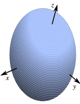
Figure 2.1 Ellipsoid representation of a general interaction tensor.
The C! term contains various constants characteristic of the ! interaction and of the
spins involved. The two three-component vectors Xˆ and Yˆ are the two interacting entities (nuclear spin operators or external sources of perturbation). The second-rank
tensor A! (a 3!3 matrix) describes the orientation dependence of the interaction
between these two vectors. It is possible to choose a frame of reference in which the
second-rank tensor A! is diagonal. This frame of reference, referred to as Principal
Axis Frame (PAF), is determined by the local environment of the nuclear sites. The
elements of the diagonalized tensor APAF are termed the principal values. Rather than
with these three values, it is common practice to characterize the tensor APAF through
the following derived parameters:
Aiso=
1
3
(
Axx+Ayy+Azz)
= 13Tr A
PAF
!" #$
(2.42)
!A =Azz"Aiso (2.43)
!A = Axx"Ayy
#A . (2.44)
Aiso, !A and !A are the isotropic component, the anisotropy and the asymmetry
respectively. As schematically depicted in Figure 2.1, an interaction tensor can be
pictured as an ellipsoid centered at the nucleus with its principal components
axis is performed acting on the tensor A! with the rotation operator Rˆ!=exp
{
"i#Lˆ!}
so to produce A!!=RˆA!Rˆ"1. Sometimes it is more convenient to express Hamiltonians
in a spherical representation:
ˆ
H! =C!
( )
"1 mAl.mTl,"m m="ll
#
l=02
#
, (2.45)where A and T are irreducible spherical tensors23 (see Appendix B) related to the
spatial and spin part respectively of the Hˆ
! Hamiltonian. Rotations on either A or T
are performed with:
!
Tl,m= Tl,mDm!,m
l
( )
(
",#,$)
m=%l l
&
, (2.46)where Dm!,m l
( ) is the element of the Wigner rotation matrix24 of rank
l:
Dm!,m l
( )
(
",#,$)
=exp{
%im!"}
d!
m,m l
( )
( )
# exp{
%im$}
, (2.47)with dm!,m l
( ) reduced Wigner elements24 (see Appendix C). The set of angles !
,",#
(
)
are Euler angles16, 24 (see Appendix D).
2.9 Average Hamiltonian Theory
The formulation of the propagator as U tˆ
( )
=exp{ }
!iHtˆ assumes a time-independentHamiltonian is acting on the spin system during the time t after which the density
matrix may be calculated. If, however, different consecutive Hamiltonians govern the
spin interactions during t, the appropriate formulation of the propagator becomes:
ˆ
U t
( )
=exp{
!iHˆntn}
exp{
!iHˆn!1tn!1}
...exp{
!iHˆ2t2}
exp{
!iHˆ1t1}
. (2.48)The calculation of an average Hamiltonian H to replace the series of exponentials
with a single U tˆ
( )
=exp{ }
!iHt does not generally yield a good descriptor of the timeevolution because the resulting density matrix subject to H would be dependent upon
the time t for which H was calculated. However, it is often the case in solid-state
NMR, that the Hamiltonian is periodic in time over a period tp. In such a
propagator U tˆ
( )
p =exp{
!iHtp}
can be used as a proper descriptor of the evolution of the density matrix over the time tp.25 When this periodicity of the spin interactions isfulfilled, the series of exponentials in Equation (2.48) can be evaluated with the
Magnus expansion:26
exp ˆ
{ }
A exp ˆ{ }
B =exp ˆA+Bˆ+ 1 2!ˆ A, ˆB
!" #$ % & ' ( ) *
exp ˆ
{ }
A exp ˆ{ }
B = + 13! ˆ
A, ˆ!" #$A, ˆB !
" #$+!"!" #$A, ˆˆ B , ˆB#$
(
)
+... % & ' ( )*, (2.49)
becoming over the period tp =t1+t2 +... tn!1+tn,
H =H(1)+ H(2)+
... (2.50)
where
H(1) = 1 tp
ˆ H t
( )
dt 0tp
!
; H(2)=! 12tp
dt2 "#H tˆ
( )
2 , ˆH t( )
1 $%dt1 0t2
&
0
tp
&
. (2.51)The first term of the series is the simple average Hamiltonian over the time tp. Higher-order terms involve commutators of the Hamiltonians at different times. Clearly, if
the Hamiltonians commute with each other at different times, only the first term of the
expansion needs to be considered for an accurate description of the density operator evolution. In the case in which the Hamiltonians operating over tp time do not
commute with each other, it is often possible to move to a rotating frame where these
non-commuting terms disappear. In this new frame of reference, called the toggling or interaction frame, the first-order term of the Magnus expansion is again a good
descriptor of the evolution of the spin system. Average Hamiltonian Theory27 (AHT)
is said to truncate the Hamiltonian to its first-order term. In order to clarify how the toggling frame removes non-commuting Hamiltonians, consider a spin system subject
to two general ! and " interactions for which the corresponding Hamiltonians Hˆ !
and Hˆ! are:
ˆ
H! =C!XˆA!!Yˆ ; Hˆ! ="!Zˆ. (2.52)
!" is the precession frequency of the Zˆ =
(
0 0 Zˆz)
spin operator andˆ
ˆ
HTot =Hˆ! +Hˆ" =C!XˆA!!Yˆ+#"Zˆ. (2.53)
The Xˆx, Xˆy, Yˆx and Yˆy components of Hˆ! do not commute with the Zˆz component
of Hˆ!. This means Hˆ! and Hˆ! do not commute with each other so that AHT needs to take into account additional terms besides the first in the Magnus expansion.
However, the transformation to the Hˆ!-toggling frame (a frame of reference rotating
at !" frequency) produces the rotating total Hamiltonian:
ˆ HTot
! =Rˆ
z "1 #
$t
( )
HˆTotRˆz
( )
#$t "#$Zˆˆ
HTot
! =Rˆ
z "1 #
$t
( )
Hˆ%Rˆz
( )
#$t +Rˆz "1 #$t
( )
Hˆ$Rˆz
( )
#$t "#$Zˆˆ
HTot
! =C
"'&exp
{
i#$tLˆz}
Xˆexp{
%i#$tLˆz}
()A!"ˆ
HTot
! =" exp i#
$tLˆz
{
}
Yˆexp %i#$tLˆz
{
}
&
' ()+#$Zˆ%#$Zˆ
ˆ HTot
! =C
"'&exp
{
i#$tLˆz}
(
Xˆx Xˆy Xˆz)
exp{
%i#$tLˆz}
()A!"ˆ
HTot
! =" exp i#
$tLˆz
{
}
Yˆx Yˆy Yˆz
(
)
exp{
%i#$tLˆz}
&
' ()
ˆ HTot
! =C
"&'Xˆxcos
( )
#$t +Xˆysin( )
#$t , ˆXycos( )
#$t %Xˆxsin( )
#$t , ˆXz()A!"ˆ
HTot
! =" Yˆ
xcos
( )
#$t +Yˆysin( )
#$t , ˆYycos( )
#$t %Yˆxsin( )
#$t , ˆYz&' (). (2.54)
The toggling frame transformation has removed the non-commuting Hˆ! Hamiltonian but has introduced time dependency. As Hˆ
! is the only interaction remaining and
commuting with itself, in the toggling frame it is possible to apply AHT to obtain the
first-order term:
HTot 1
( ) = 1
tp ˆ HTot ! dt 0 tp
"
=C#XˆzA!#,zzYˆz. (2.55)All the time dependent cos- and sin-modulated terms integrate to zero over tp, leaving
the only non-modulated z-components of the spin operators as these are not affected
by the Lˆz rotation operator through which the frame rotation itself was achieved.
AHT produces therefore a much simpler formulation of Hamiltonians which are said
2.10 The magnetic field
The NMR phenomenon is based upon the effect of an external magnetic field B0
upon I !0 nuclei.28 This interaction is called Zeeman effect and the Hamiltonian which describes it is the Zeeman Hamiltonian HˆZ, expressed in Cartesian coordinates as:
ˆ
HZ =!"Iˆˆ1B0
ˆ
HZ =!"
(
Ix Iy Iz)
1 0 0 0 1 0 0 0 1
# $ % % & ' ( (
B0x
B0y
B0z # $ % %% & ' (
((. (2.56)
By convention, the external magnetic field is applied along the z-axis of the
laboratory frame of reference simplifying the Hamiltonian to:
ˆ
HZ =!"
(
Ix Iy Iz)
1 0 0 0 1 0 0 0 1
# $ % % & ' ( ( 0 0 B0 # $ % % & ' ( ( ˆ
HZ =!"IˆzB0 =#0Iˆz. (2.57)
The term !"B0 =#0 is referred to as the Larmor frequency. When placed in an external magnetic field, a I!0 spin magnetic moment is found to precess about the field direction at a frequency
!
0. The Hamiltonian HˆZ acting on the spinwavefunction I,m returns the eigenvalues associated with the energy levels
available:
ˆ
HZ I,m =!0Iˆz I,m . (2.58)
Since HˆZ and Iˆz commute with each other ([HˆZ, ˆIz] = 0), they result in the same eigenfunctions I,m . Considering that Iˆz I,m =m I,m ,
ˆ
HZ I,m =!0m I,m (2.59)
so that the energy of the eigenstates is Em=m!0. For a nucleus with spin quantum
number I = 1/2 with the two ! and " states |1/2, +1/2! and |1/2, "1/2!, the energy
resonance occurs when the spin system, placed into an external magnetic field, is
supplied an amount of energy that matches that associated with the Larmor frequency.
2.11 Pulses
The only way the spectroscopist can manipulate the magnetization arising from an
ensemble of spins in a B0 magnetic field is through the B1 magnetic component of electromagnetic pulses.28 Given the usual strength of modern superconducting
magnets, these pulses fall into the radiofrequency (rf) region of the electromagnetic
spectrum. Pulses are applied through a coil surrounding the sample in a geometric
manner such that the magnetic components of the pulses are perpendicular to the
external field (i.e., in the xy-plane of the laboratory frame of reference). The
Hamiltonian governing the interaction between the spin operators and a pulse of
strength B1 applied along the x-axis of the laboratory frame is, in analogy with the
Zeeman Hamiltonian, given by:
ˆ
Hrf =!"Iˆxˆ1B1
ˆ
Hrf =!"
(
Ix 0 0)
1 0 0 0 1 0 0 0 1
# $ % % & ' ( ( B1 0 0 # $ % % & ' (
(. (2.60)
However, this would be the case if the B1 magnetic field was, as with B0, static.
Being intrinsically connected to the electromagnetic pulse, B1 oscillates along the
x-axis with a modulation described by a cos(!rft) term, where !rf is the frequency of
the electromagnetic wave. Therefore, in the laboratory frame of reference, the
Figure 2.2 Effect of a !y pulse on the z-magnetization in the Zeeman frame. The B1 field and the
pathway followed by the magnetization under the effect of the pulse are indicated in red.
ˆ
Hrf =!"IˆxB1cos(#rft). (2.61)
The oscillating amplitude of B1 can be thought of as a vectorial sum of two
counter-rotating fields:
ˆ
Hrf =! 1
2"B1 exp !i#rft ˆ
Iz
{
}
Iˆxexp
{
i#rftIˆz}
(
)
ˆ
Hrf =!
1
2"B1 exp i#rft ˆ Iz
{
}
Iˆxexp
{
!i#rftIˆz}
(
)
. (2.62)The first term rotates at !rf whereas the second field rotates at !"rf. If !rf
approaches !0 the component rotating at !"rf can be ignored as it is too far off
resonance to affect the spin. Omitting the 1/2 factor, the Hamiltonian therefore
becomes:
ˆ
Hrf =!"B1
(
exp{
!i#rftIˆz}
Iˆxexp{
i#rftIˆz}
)
. (2.63)Since the spin operators satisfy all the cyclic permutations of commutators [Iˆz, ˆIx] =
iIˆy, Hˆrf can also be expressed as:
ˆ
In order to eliminate the time dependency of the pulse Hamiltonian, a transformation
to a frame rotating at !rf around the z-axis can be performed with the rotation
operator Rˆ
z =exp
{
!i"rftIˆz}
acting on Hˆrf. Considering Equation (2.63), theinteraction frame Hamiltonian Hˆrf
! is expressed as:
ˆ
Hrf ! =Rˆ
zHˆrfRˆz "1
ˆ
Hrf
! ="#B
1%&exp
{
i$rftIˆz}
(
exp{
"i$rftIˆz}
Iˆxexp{
i$rftIˆz}
)
exp{
"i$rftIˆz}
'(ˆ
Hrf
! ="#
B1Iˆx =$1Iˆx. (2.65)
The toggling-frame pulse Hamiltonian becomes therefore time independent and !1 ="#B1 is the frequency of nutation imposed by the pulse upon the magnetization. In Figure 2.2 a schematic representation of the effect of a y-pulse is depicted. The angle through which the magnetization nutates under the torque imposed by the pulse
is ! ="1t. The interaction frame transformation is possible because the
time-dependent Schrödinger equation d ! /dt="iHˆ ! is invariant to frame
transformations.16, 29 Introducing a !R wavefunction corresponding to a !
rotating around the z-axis:
!R =exp
{
i"rftIˆz}
! or ! =exp{
"i#rftIˆz}
!R , (2.66)the time dependency of !R is expressed by:
d !R
dt =i"rf ˆ
Izexp
{
i"rftIˆz}
! +exp{
i"rftIˆz}
d !
dt
d !R
dt =i"rf ˆ
Iz !R +exp
{
i"rftIˆz}
(
#iHˆ !)
d !R
dt =i"rf ˆ
Iz !R +exp
{
i"rftIˆz}
(
#iHˆexp{
#i"rftIˆz}
!R)
d !R
dt ="i "#rf
ˆ
Iz +exp
{
i#rftIˆz}
Hˆ exp{
"i#rftIˆz}
$
% &' !R
d !R
dt ="i "#rf
ˆ
Iz +RˆzHˆRˆz
"1
$% &' !R
d !R dt ="i
ˆ
The rotating HˆR is made up of the original Hˆ subject to the same rotation of the wavefunction !R and the !"rfIˆz term which governs the rotation itself. Considering the total Hamiltonian in the laboratory frame during a pulse
ˆ
HLab =HˆZ+Hˆrf , its interaction frame representation Hˆ
! Lab is:
ˆ
H!Lab="#rfIˆz+RˆzHˆLabRˆz
"1
ˆ
H!Lab ="#rfIˆz +exp
{
i#rftIˆz}
(
HˆZ +Hˆrf)
exp{
"i#rftIˆz}
ˆ
H!Lab ="#rfIˆz +exp
{
i#rftIˆz}
(
#0Iˆz+#1%$exp{
"i#rftIˆz}
Iˆxexp{
i#rftIˆz}
&')
ˆ
H!Lab ="exp
{
#i$rftIˆz}
. (2.68)The Rˆz rotation operator does not have any effect on the Iˆz term, therefore:
ˆ
H!Lab ="#rfIˆz +#0Iˆz +#1%$exp
{
i#rftIˆz}
(
exp{
"i#rftIˆz}
Iˆxexp{
i#rftIˆz}
)
&'ˆ
H!Lab ="exp
{
#i$rftIˆz}
%&ˆ
H!Lab =
(
"0 #"rf)
Iˆz +"1Iˆx ˆH!Lab ="Iˆz+#1Iˆx (2.69)
The parameter !="0#"rf is referred to as the offset. For an on-resonance pulse (!0 =!rf) the pulse-frame total Hamiltonian is reduced to that of Equation (2.65). For
an on-resonance pulse therefore, in the toggling frame, the effect of the static magnetic field B0 vanishes.
2.12 The chemical shielding
Given an external magnetic field B0, from the definition of the Zeeman Hamiltonian ˆ
HZ in Equation (2.57), all nuclei with the same gyromagnetic ratio ! should
to as chemical shielding.30 This means, for example, that all the 1H in a given system
have different resonance frequencies, according to their different chemical
environment. The Cartesian Hamiltonian of this interaction is expressed in its PAF
by:
ˆ
HCS =!Iˆ"!B0
ˆ
HCS =!
(
Iˆx Iˆy Iˆz)
"xx PAF
0 0
0 "yy PAF
0 0 0 "zz PAF # $ % % % & ' ( ( ( 0 0 B0 # $ % % & ' (
(. (2.70)
The principal components of the shielding tensor !! in its PAF are commonly
expressed in terms of the isotropic shielding !iso, shielding anisotropy !CS and
asymmetry !CS, defined as:
!iso = 1
3 !xx PAF +!
yy PAF +!
zz PAF
(
)
= 13Tr !! PAF
"# $% (2.71) !CS ="zz
PAF #"
iso (2.72)
!CS ="xx PAF#"
yy PAF
$CS
. (2.73)
The first-order truncated average Hamiltonian in the rotating frame is:
ˆ
HCS =!Iˆz"zz Lab
B0. (2.74)
The term !zz
Lab is related to the principal components of the shielding tensor in the
PAF by:
!zz Lab =!
iso+
1
2"CS 3cos 2#$
1+%CSsin
2#
CScos 2&CS
(
)
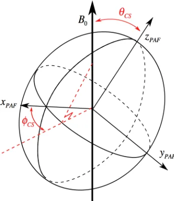
, (2.75)where !CS and !CS are the polar angles which relate the orientation of the external
magnetic field to that of the shielding tensor in its PAF, as shown in Figure 2.3. A
third angle is redundant as it has no influence on the value of !zz
Lab. It is possible to
Figure 2.3 Orientation of the external magnetic field in the PAF shielding ellipsoid as defined
by the two polar angles !CS and "CS depicted in red.
E I,m =HˆCS I,m
E I,m =!Iˆz"zz Lab
B0 I,m (2.76)
E I,m I,m =! I,m Iˆz I,m "zz Lab
B0 (2.77)
E=! I,m Iˆz I,m
I,m I,m "zz
Lab
B0
E=! Iˆz "zz Lab
B0
E=!m"0#zz Lab ="
CS m
( ). (2.78)
The |1/2, +1/2! " |1/2, #1/2! transition frequency is therefore:
!CS " #$ =!
CS %1/2
( )%!
CS 1/2
( )=!
0&zz
Lab. (2.79)
Equation (1.80) shows that the electrons perturb the Larmor frequency resonance
condition experienced by a bare nucleus by the factor !zz
Lab. Equation (2.79) also
shows how the measurement of the shielding interaction of a given spin yields
information directly related to the electronic or chemical environment of the nuclear
sites. The dependence of the chemical shielding interaction upon the magnetic field
resonance phenomenon at a frequency which is proportional to the field strength
itself. In order to compare data acquired on different spectrometers, i.e., at different
fields, rather than quoting the frequency of resonance of spins in Hz, the concept of
chemical shift ! has been introduced and defined as:31
! =106" # "standard
"standard
, (2.80)
where " is the frequency of resonance of the spin with chemical shift ! and "standard is
the frequency of resonance of a standard spin whose chemical shift !standard is
arbitrarily set to zero. The chemical shift is a dimensionless descriptor and is quoted in parts per million, or ppm, by virtue of the 106 factor which simply scales up the chemical shift to more convenient values.
2.13 Multispin systems
The interactions so far described are related to single-spin systems. There are other interactions however which involve perturbations caused by other spins. When n-spin systems have to be described, the required Hamiltonian is the sum of all the i-th Hamiltonians:16
ˆ
H!Sys = ˆ
H!,i
i=1 n
"
. (2.81)The wavefunction associated with the n-spin system is the product of all the i-th single-spin wavefunctions:
ISys,mSys = Ii,mi i=1
n
!
(2.82)such that, for example, for a I and S two-spin system the wavefunction is:
II,mI IS,mS = II,mI;IS,mS . (2.83)
The Zeeman states have energies:
E ISys,mSys = HˆZ Sys
ISys,mSys (2.84)
E ISys,mSys ISys,mSys =!0 ISys,mSys Iˆz,i i=1
n
E=!0 Iˆz,i i=1
n
"
E=!0 mi i=1
n
"
. (2.86)Since the azimuthal quantum number m varies between –I and +I in steps of 1, for an
n-spin system the number of available spin eigenstates is (2I+1)n. This allows the
existence of MQ transitions even for I = 1/2 nuclei.
2.14 The dipolar coupling
The dipolar coupling arises from the through-space interaction of nuclear magnetic
moments.32 Classically, this coupling can be visualized as the interaction between
pairs of bar magnets. Being a through-space mechanism, the dipolar coupling supplies
information about both inter- and intra-molecular proximity. In the Cartesian
representation the Hamiltonian associated with this interaction in its PAF is given by:
ˆ
HD =!2 ˆID!Sˆ
ˆ
HD =!2 ˆ
(
Ix Iˆy Iˆz)
Dxx PAF
0 0
0 Dyy PAF
0 0 0 Dzz PAF " # $ $ $ % & ' ' ' ˆ Sx ˆ Sy ˆ Sz " # $ $ $ % & ' '
'. (2.87)
The D! tensor is traceless (Tr[D!] = 0) so there is no isotropic component. This means
in the solution phase the rapid molecular tumbling averages this interaction to zero. !
D is also always axially symmetric, with its unique axis lying along the I-S vector. Its
principal components are Dxx PAF =
Dyy PAF =!
dIS / 2 and Dzz PAF =
dIS, with dIS termed
dipolar coupling constant and expressed by:
dIS =
!µ0
4! 1
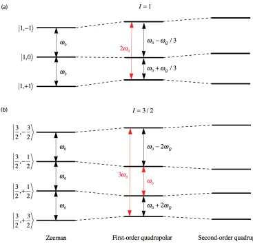
Figure 2.4 Effect of the dipolar coupling interaction on the Zeeman eigenstates. In (a) a heteronuclear couple of spins is considered. In (b) a homonuclear couple of spins is considered. In (c) a homonuclear system of M spins is considered. Only the transitions associated to one spin are shown in each case.
Equation (2.88) shows the through-space dependence of HˆD upon r
!3. The dipolar
interaction therefore can produce important spatial information about spins regardless
of the presence of a chemical bond between them. For the case of a heteronuclear spin
pair, the first-order averaged Hamiltonian is truncated to:
ˆ HD
Het =!
dIS 3cos 2" !
1
(
)
IˆzSˆz. (2.89)
For a I-S two-spin system, the Zeeman states are therefore affected by the dipolar
coupling constant dIS by II,mI;IS,mS IˆzSˆz II,mI;IS,mS =mImS. In the case of I = S
= 1/2 nuclei, the |!!!, |!"!, |"!! and |""! states have energy-shift factors of +1/4, –
1/4, –1/4 and +1/4 respectively. In the homonuclear case the |!"! and |"!! states are
degenerate and the truncated Hamiltonian is given by:
ˆ HD
Hom =!d
IS 3cos
2" !
1
(
)
IˆzSˆz ! 1 2
ˆ
IxSˆx+IˆySˆy
(
)
# $%
&
'(. (2.90)
The most important implication which results from the additional Iˆ
xSˆx and IˆySˆy terms is that the degenerate |!"! and |"!! product wavefunctions are not eigenfunctions of
these operators.33 Eigenfunctions of the IˆxSˆx and IˆySˆy operators for the two
degenerate states have to be expressed as linear combinations of the |!"! and |"!!