Vol. 12, No. 2, pp 321-334
A GLM-Based Method to Estimate a Copula’s
Parameter(s)
Amir T. Payandeh Najafabadi1, Mohammad R. Farid-Rohani1,
Marjan Qazvini2
1Mathematical Sciences Department, Shahid Beheshti University, G.C. Iran. 2E.C.O College of Insurance, Allameh Tabatab´ai University, Iran.
Abstract. This study introduces a new approach to problem of
esti-mating parameter(s) of a given copula. More precisely, using the con-cept of the generalized linear models (GLM) accompanied with least square method, we introduce an estimation method, say GLM-method. A simulation study has been conducted to provide a comparison among the inversion of Kendal’s tau, the inversion of Spearman’s rho, the PML, the Copula-quantile regression with (q = 0.25,0.50,0.75), and the GLM-method. Such simulation study shows that the GLM-method is an ap-propriate method whenever the data distributed according to an ellipti-cal distribution.
Keywords. Copula, copula-quantile regression, GLM, parameter
esti-mation.
MSC: 62F10, 62J05, 62J12, 62H20.
1
Introduction
Copula is used to model the relationship between random variables. It can capture the interdependency that cannot be exhibited by other as-sociation measures such as the well-known correlation coefficient. One
Amir T. Payandeh Najafabadi( )([email protected]), Mohammad R. Farid-Rohani([email protected]), Marjan Qazvini([email protected]) Received: November 2012; Accepted: June 2013
step in copula modeling is the estimation of parameters. The most ef-ficient method is the maximum likelihood estimator (MLE), which is used to evaluate the parameter of any kind of models. It can also be applied to copula, but the problem becomes complicated as the number of parameters and dimension of copula increases, because the parame-ters of the margins and copula are estimated simultaneously. Therefore, MLE is highly affected by misspecification of marginal distributions. A rather straightforward way at the cost of lack of efficiency is inference-functions for margins (IFM), which is put forward by Joe (2005). The idea of this method came from psychometrics literature for latent models based on the multivariate normal distributions. Similar to MLE in this method the margins of the copula are important, because the parame-ter estimation is dependent on the choice of the marginal distributions. First the margins’ parameters are estimated and then the parameters of copula will be evaluated given the values from the first step.The ef-ficiency of this method is 1 for product copula under some conditions. Efficiency decreases with strong dependence. IFM is not a good estima-tion technique due to its efficiency for extreme dependence near Fr´echet bounds. Both MLE and IFM are placed in the category of parametric methods. Genest et. al. (1995) introduce a semiparametric method, known as maximum pseudolikelihood estimation (mpl), similar to MLE. The only difference between this method and MLE is that the data must be converted to pseudo observations. The consistency, asymptotic normality of this method is established in their paper. They established that this method is efficient for independent copula. Two nonparametric methods based on the rank of observations are inversion of Kendall’s tau (itau) and Spearman’s rho (irho). These moment estimations are applied to one parameter copula when it is exchangeable (Kojadinovic & Yan, 2010). Kojadinovic & Yan (2010) found that whenτ ≤0.4, the inversion of Spearman’s rho is a good approach for estimating the parameter of Gumbel-Hougaard copula. They compared mpl, irho and itau by look-ing at their mean square error, for different sample sizes and dependency level. It turns out that for n= 50 and τ ≤ 0.2 i.e. weak dependency, two methods of moment estimation seem to be better than the esti-mation based on pseudo likelihood. However, as dependency increases and sample size gets larger, mean square error for mpl will reduce. The estimation based on mpl is more biased than the methods of moment estimators, but the biasedness will decrease as n gets larger. The esti-mation based on the inversion of Spearman’s rho performs well for the Gumbel-Hougaard copula. In general, the estimation based on Kendall’s
tau is better than the Spearman’s rho. Tsukahara (2005) introduced a semiparametric estimator, known as “rank approximate Z-estimator”. He also proved the asymptotic normality of this estimator. Through a Monte Carlo simulation, he compared τ-inversion, ρ-inversion, PML, minimum Cram´er-von Mises distance, minimum Kolmogorov-Smirnov distance and rank approximate Z-estimators. He concluded that PML has the lowest MSE and Z-estimator has the lowest bias. Vandenhende & Lambert (2005), showed that it was possible to form a univariate distribution from any Archimedean copula (see Theorem 1) by writing the generating function in linear form. They used least square esti-mation to evaluate the copula parameters. Brahimi & Necir (2012), evaluated the parameters of copula using method of moments. They particularly focused on Archimedean copulas. Consistency and asymp-totic normality of their procedures have been verified. They concluded that their method is practically faster and easier. Qu et al. (2009) used the fact that a multivariate Archimedean copula is the same as survival copula of multivariate L1-norm symmetric distributions and proposed a method for parameter estimation and model selection concentrating on Archimedean families. They established the consistency of the esti-mator and applied Radia Information Criteria (RIC) for selecting the well-fitted Archimedean copula. Kim et al. (2007) compared two para-metric estimation methods i.e. MLE and IFM with PML. They showed that misspecification of margins had significant impact on parameter estimation when the methods used were IFM and MLE. But PML is ro-bust against margins misspecification, therefore it is preferred to other two methods. However, MLE is the most efficient method and at the same time the most efficient one when dealing with multivariate multi parameter copulas. They advised on using PML method. de Haan et al. (2008) calculated the parameter of extreme value copula for censored data using pseudo-sample based on MLE. The asymptotic distribution of this method was established in their paper. They also proposed a test statistic for selection of the appropriate copula and found its critical values using bootstrap methods.
This study uses the concept of the generalized linear model (GLM) along with the least square method and introduces a new estimation method, namely GLM-method, for estimating parameter(s) of a given copula. Performance of such GLM-method is compared with perfor-mance of other estimation methods through a simulation study. Cram´ er-von Mises distance is employed as a criteria for such comparison. This article is organized as follows: Section 2 provides a brief review on
rameter estimation methods and considers copula quantile regression. GLM-method introduces in Section 3. Section 4 compares different methods of calculating copulas’ parameters through a simulation study, and Section 5 concludes.
2
Methods of Parameter Estimation
This section reviews some most applicable methods used for parameter estimation of a given copula. As explained above although MLE is misspecified by the margins, it is the most efficient method, which can be implemented by
L(Θ) =
T
∑
t=1
lnc(F1(x1t), F2(x2t), . . . , Fd(xdt)) + T
∑
t=1
d
∑
j=1
lnfj(xjt),
where Θ is the vector of all parameters of both the marginals and the copula, andcis ∂Cθ(F1(t1),...,Fd(td))
∂F1(t1)...∂Fd(td) . Another parametric method is IFM,
where first the parameter of the margins are estimated and then the parameters of the copula, namely
L(α, θ1, . . . , θn) = m
∑
i=1
logf(xi;θ1, . . . , θn, α).
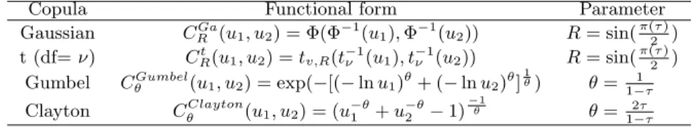
The point estimation methods i.e. itau and irho are two nonparametric methods, which are applied given the relationship between the parame-ter of the copula and the Kendall’s tau and Spearman’s rho association measures viz. θ=g−1(τ). Such relationship is presented in Table 5 .
Table 1: Two dimensional Copulas, the relations between parameters and Kendall’s tau, τ.
Copula Functional form Parameter Gaussian CRGa(u1, u2) = Φ(Φ−1(u1),Φ−1(u2)) R= sin(π(2τ))
t (df=ν) Ct
R(u1, u2) =tv,R(t−ν1(u1), t−ν1(u2)) R= sin(π(2τ))
Gumbel CθGumbel(u1, u2) = exp(−[(−lnu1)θ+ (−lnu2)θ] 1
θ) θ= 1
1−τ
Clayton CθClayton(u1, u2) = (u−1θ+u−
θ
2 −1)
−1
θ θ= 2τ
1−τ
The nonparametric version of MLE, which seems to perform better than other methods when the sample size and level of dependence increases is PML, in which the data must be converted to pseudo observations. Suppose Xi = (Xi,1, . . . , Xi,p) are random vectors and Rij the rank
of Xij. Then by applying ˆUij = nR+1ij the pseudo observations can be
calculated. Therefore, the pseudo log-likelihood is given by logL(θ) =
n
∑
i=1
logcθ( ˆui),
where ˆui= ( ˆUi,1, . . . ,Uˆi,p). For a bivariate copula this simplifies to
L(θ) =
n
∑
i=1
log{cθ(
Ri
n+ 1, Si
n+ 1)}.
2.1 Copula-Quantile Regression
When the distribution function of the variables is not normal, the con-ditional expectation E(Y|X) and conditional variationV ar(Y|X) does not suffice to give full information on the conditional distribution func-tion. In such cases, the quantile regression is used. To estimate the parameters of the quantile regression LSE can be applied, however as opposed to standard mean regression, the loss function is not square error, instead it is the absolute error loss function, hence the sign of the error terms is important (Alexander, § 7, 2008). Copula-quantile regression, which is introduced by Bouy´e & Salmon (2009) is a non-linear form of quantile regression. To apply quantile regression, one needs to know the conditional copula distribution which is given by CU|V(u|v) = ∂v∂C(u, v), CV|U(v|u) = ∂u∂ C(u, v). The copula-quantile
regression is defined as the following.
Definition 2.1. IfC(., ., θ) is a parametric copula with parameter θ,
the pth quantile curve ofv conditional onu is defined by p= ∂C(u, v;θ)
∂u ,
and rearranging with respect tovthe copula-quantile regression is given by
v=r(u, p;θ).
They studied properties of copula-quantile regression and showed its application on the interdependency between foreign exchange markets, which are skewed. They also compared their findings with tail depen-dency measure at differentα. They noted that tail dependency at differ-entαis not corresponding to copula regression at different quantiles and
the results are different. They expressed that their results were more reliable. The following lemma utilized from Bouy´e & Salmon (2009)’s finding and established the expression of quantile regression for 5 most applicable copulas, i.e., Clayton, Frank, Gumbel, Normal, and t copulas.
Lemma 2.1. (Bouy´e & Salmon, 2009) The copula-quantile regression
for different class of copulas is given by
(i) Clayton copula v= ((p−θ/(1+θ)−1)u−θ+ 1)−1/θ;
(ii) Frank copula v= −θ1ln(1−(1−e−θ)(1 +e−θu(p−1−1))−1);
(iii) Normal copulav= Φ(ρΦ−1(u) +√1−ρ2Φ−1(p));
(iv) t-copulav=tν(ρt−ν1(u)+
√
(1−ρ2)(ν+ 1)−1(ν+t−1
ν (u)2)t−ν+11 (p)). To employ the above lemma, one has to set u := FX(x) and v :=
FY(y). It should be worthwhile to mention that the Gumbel copula
does not have a closed form for the copula-quantile regression method. Therefore, its copula-quantile regression has to be found numerically.
3
GLM Approach to Parameter Estimation
The idea of using the GLM method for estimating parameter(s) of a given copula has been suggested roughly by several authors, see Genest (1987) and Frees & Valdez (1998) for Frank copula; Parsa & Klugman (2011) for Gaussian copula.
The following theorem uses the GLM method along with the least square method and provides a particle algorithm to estimate copula’s parameter(s).
Theorem 3.1. SupposeC(., ., θ) is a bivariate copula function with
parameterθ.Then, based upon continuous random sample (X1, Y1),(X2,
Y2),· · · ,(Xn, Yn), copula parameter θ can be estimated by minimizing
the following least square function inθ.
Q(θ) =
n
∑
i=1 (
Vi−1 +
∫ 1 0
∫ k
0
cθ(Ui, t)dtdk
)2
, (1)
whereVi :=FY(Yi) andUi:=FX(Xi).
Proof. The GLM expression on two uniform random variables V and U can be stated as
E(V|U =u) =
∫ ∞
0
(1−FV|U(v|u))dv+ ∫ 0
−∞FV|U(k|u)dk
= 1− ∫ 1
0
FV|U(k|u)dk
= 1− ∫ 1
0 ∫ k
0
fU,V(u, t)
fU(u)
dtdk
= 1− 1
cθ0(u)
∫ 1 0
∫ k
0
cθ(u, t)fV(t)dtdk
= 1− ∫ 1
0 ∫ k
0
cθ(u, t)dtdk.
The second and last equations arrived from the fact thatV andUare two uniform random variables and the forth equation arrives from identity f(t1, . . . , td) =cθ(F1(t1), . . . , Fd(td))
∏d
i=1fi(ti).
Now the least square expression can be written as Eqution 1. In most cases the above theorem has to be employed numerically. The following corollary explores a situation that the GLM-method has explicit solution.
Corollary 3.1. Supposecθ(·,·) is a Farlie-Gumbel-Morgenstern
cop-ula function. Then, using random sample (X1, Y1),(X2, Y2),· · · ,(Xn, Yn),
copula parameterθ is θ = 3
∑n
i=1(yi−12)(xi−12)
∑n
i=1(xi−12)2
.
Proof. The PDF of Farlie-Gumbel-Morgenstern copula is
cθ(u, v) = 1 +θ(1−2u)(1−2v).
Substitutingcθ(u, v) is least square function given by Theorem 3.1 leads
to
Q(θ) =
n
∑
i=1
(yi−1 +
1 2+
1
6θ(1−2xi))
2.
The desire proof arrives after solving ∂θ∂Q(θ) = 0 in θ.
The copula’s PDF, cθ(·,·),plays a crucial role in calculation of
E(V|U =u) = 1− ∫ 1
0 ∫ k
0
cθ(u, t)dtdk,
in Theorem 3.1. Table 2 provides the copula’s PDF,cθ(·,·) for some well
known class of copulas.
4
Simulation Study
Now a simulation study compares these five estimation methods numer-ically. For this propose five different distributions normal, t, Cauchy, and two extreme value distributions, logistic and H¨usler-Reiss distri-butions are selected. The first three distridistri-butions are symmetric and appropriate for financial data and the last two are appropriate distribu-tions for insurance and reinsurance portfolios, which involve losses with high severity and low frequency. The distribution of insurance claims data are normally skewed and heavy-tailed (Embrechts et el., 2002, and Kotz & Nadarajah, 2000). The data are simulated from these distribu-tions with high dependence level at 0.9. All data are transformed into pseudo-observations. First, they are ranked and then multiplied by n+11 to avoid problem that may arise at boundary [0,1]d. Five copulas, which are mostly used, viz, Gumbel, Frank, Clayton, normal and t copulas are selected. The parameters are estimated with 5 approaches: (i) Inver-sion of Kendal’s tau; (ii) Inversion of Spearman’s rho; (iii) PML; (iv) Copula-quantile regression with (q = 0.25,0.50,0.75), and (v) GLM-method. It is expected that each method is suitable for a particular distribution. To compare the results, the cram´er-von Mises distance is used. It is defined by
∫ ∞
−∞
∫ ∞
−∞(FXY(x, y)−Cθ(FX(x), FY(y)))
2f
XY(x, y)dxdy.
This criteria measures how far is the distance of the real data from the data generated by copula; in other words, this is the weighted average of the errors. Normally the lower this distance, the better would be the results. The simulation is carried out on sample size 1000 with 100 iterations using the packages copula,fCopulae, quantreg, andevd in R. The calculation for elliptical copulas and distributions take longer than others. The results are presented in the tables below.
The tables present the mean and standard deviation for parameters of different copulas and their corresponding Cram´er distance. The first table is based on the data generated from Logistic distribution, which is an extreme value distribution function. For this distribution, when the copulas are Clayton and Gumbel, PML gives better result. For other copulas, quantile regression method dominates other approaches.
Copula-quantile regression at 50%,25% and 50% performs better than other methods when the underlying copulas are Frank, Normal and t (df=4), respectively. However, the results obtained by different meth-ods is not significantly different when copulas are elliptical. The second table shows the results for H¨usler-Reiss distribution, which is another extreme value distribution function under study. Similar to Logistic distribution, the performance of PML is better than other approaches when the copulas are Clayton and Gumbel. Moreover, when the copula is Frank, quantile regression at 25% gives better result. Although not significantly different, the Cram´er distance given by irho is lower than copula-quantile regression at 75% when the copula is normal. GLM per-forms well when copula is t. Three other distributions from which the data are simulated are elliptical. The third table belongs to the data generated from Cauchy distribution, which is also a heavy-tailed distri-bution function. Inverse of Spearman’s rho with Clayton copula does better than other estimation methods. Inverse of Kendall’s tau performs well when the copula is Gumbel. GLM supersedes other approaches when the copulas are Frank and t. The Cram´er distance obtained by different methods is roughly the same when the copula is normal. For two other elliptical distributions i.e. normal and t distributions, the performance of the estimation methods with the corresponding copulas is the same. The only difference is that for normally distributed data, itau performs better than irho when the copula is Clayton. In general, the copula-quantile regression is a better approach when the data are heavy-tailed and the GLM gives rise to better result when the data are elliptically distributed. However, with the latter the performance is the worst when copula is Gumbel regardless of the type of data.Finally, one can conclude that the estimation methods are more dependent on the type of data than the chosen copula. Therefore, it is suggested to check the data and their distributions and then pick a method that is supposed to perform better than other methods.
5
Conclusion
Copulas’ parameter estimation is the first step in copula modeling. In this study, for the first time, to the best of the authors’ knowledge, the copula-quantile regression is included in a simulation study that compares different approaches for parameter evaluation. As is expected such method is only a good approach when data are from extreme value distributions. Also a new method which is based on GLM is proposed
T able 2: CDF and PDF of tw o dimensional Copulas. Copula CDF PDF Gaussian Φ(Φ − 1( u1 ) , Φ − 1( u2 )) 1 √ 1 − θ 2 exp { − θ 2ξ 2 1−
2 θ ξ1 ξ2 + θ 2ξ 2 2 2(1 − θ 2) } t (df= ν ) tv ,R ( t − 1 ν ( u1 ) , t − 1 ν ( u2 )) 1 √ θ Γ( ν / 2+1)Γ( ν / 2) Γ( ν / 2+1 / 2) 2 [ ν (1 − θ 2)(1+ ς
2 1/ν
)(1+
ς
2 2/ν
) ν (1 − θ 2)+ ς
2 1+
ς
2 2−
2
θ
ς1 ς2
](ν
/ 2+1) Gum b el exp { − [( − ln u1 ) θ + ( − ln u2 ) θ] 1 θ } ( A + θ − 1) A 1 − 2 θ exp( − A )( xt ) − 1 Cla yton ( u − θ 1 + u − θ 2 − 1) − 1 θ 1+ θ ( xt ) θ +1 ( x − θ + t − θ− 1) − 2 − 1 /θ F rank − 1 θ ln(1 + (exp( − θ u1 ) − 1)(exp( − θ u2 ) − 1 exp( − θ ) − 1 ) exp {− θ ( x + t ) } (1 − exp {− θ } ) (exp { θ ( x + t ) }− exp {− θ x }− exp {− θ t } +exp {− θ } ) 2 where A = (( − ln x ) θ + ( − ln t ) θ) 1 /θ , ξ1 = Φ − 1( x ) and ξ2 = Φ − 1( t ) are the quan tiles of standard normal distribution, and ς1 = t − 1 ν ( x ) and ς2 = t − 1 ν ( t ) are the quan tiles of studen t distribution with ν degree of freedom. T able 3: The mean and (sd) for parameter (1st ro w) and Cram ´er distance (2nd ro w) based on differen t metho ds and differen t copulas Logistic Cla yton F rank Gum b el Normal t (df=4) itau 0.2357896 (0.04758373) 0.9549693 (0.1757497) 1.107067 (0.0292168) 0.1642097 (0.02938949) 0.1642097 (0.02938949) 0.0003710279 (0.0003495556) 0.0002174217 (0.0002381969) 76638e-05 (0.0001018399) 0.579039 (0.02567358) 0.6560563 (0.02580707) irho 0.2338561 (0.04714266) 0.9471112 (0.1742059) 1.107806 (0.02868843) 0.1629714 (0.02918711) 0.1629714 (0.02918711) 0.0003569152 (0.0003406244) 0.0002070756 (0.0002300933) 7.428632e-05 (0.0001018399) 0.5783464 (0.02557629) 0.6553711 (0.02571474) mpl 0.1379168 (0.03819629) 0.96518 (0.1761349) 1.111834 (0.02539398) 0.170902 (0.02850896) 0.1510195 (0.02719727) 8.43965e-05 (0.0001237738) 0.0002299379 (0.0002474306) 5.685229e-05 (8.676336e-05) 0.5827182 (0.02535498) 0.64889 (0.02446221) q(0.25) 3.26151 (0.1628287) 0.9533234 (0.2298271) 1.048115 (0.01800756) 0.152806 (0.04361077) 0.1826987 (0.05319693) 0.07143315 (0.002748488) 0.0002694946 (0.0002294357) 0.0004259352 (0.0002452429) 0.5737317 (0.02902004) 0.6684247 (0.03596833) q(0.50) 5.496151 (0.4657097) 0.8908815 (0.1989322) 1.050184 (0.01465274) 0.1688641 (0.03974894) 0.1366404 (0.0341501) 0.09836826 (0.003908395) 0.0001733166 (0.0002426908) 7.76638e-05 (0.0001830703) 0.5822645 (0.02910009) 0.6419208 (0.02552031) q(0.75) 3.848151 (0.2425259) 1.053014 (0.1889862) 1.052381 (0.01401862) 0.1777977 (0.03607364) 0.1978619 (0.03694576) 0.08043742 (0.003343596) 0.0003670748 (0.0003141369) 0.000358005 (0.0001654764) 0.5872107 (0.02965161) 0.6761877 (0.03174102) GLM 0.3045018 (0.06306191) 1.072397 (0.1985979) 0.3806179 (0.3222072) 0.2045057 (0.03607838) 0.2167632 (0.004406308) 0.001039189 (0.0007416712) 0.0004081506 (0.0003793207) 0.08743481 (0.05128618) 0.603464 (0.03105044) 0.6866389 (0.02079485) T able 4: The mean and (sd) for parameter(1st ro w) and Cram ´er distance (2nd ro w) based on differen t metho ds and differen t copulas H ¨usler-Reiss Cla yton F rank Gum b el Normal t (df=4) itau 0.5361688 (0.06593831) 1.971938 (0.2056333) 1.261172 (0.03080665) 0.3250657 (0.03023427) 0.3250657 (0.03023427) 0.001006468 (0.0006577236) 0.0005220021 (0.0004315309) 6.052187e-05 (7.3808e-05) 0.6646245 (0.03571358) 0.7410599 (0.03551979) irho 0.5341152 (0.0658127) 1.955466 (0.2013865) 1.260534 (0.0310642) 0.3231768 (0.02983328) 0.3231768 (0.02983328) 0.0009869564 (0.0006519294) 0.0004873584 (0.0004087076) 6.145837e-05 (7.342551e-05) 0.6627463 (0.03520841) 0.7392119 (0.03502771) mpl 0.3179717 (0.04836689) 1.988077 (0.2064492) 1.263038 (0.02907468) 0.3409704 (0.02758792) 0.3005748 (0.02937067) 0.0001601931 (0.000182298) 0.0005542253 (0.000445662) 5.429113e-05 (7.029836e-05) 0.6803328 (0.03574465) 0.7184925 (0.03246757) q(0.25) 3.915307 (0.2113648) 1.853813 (0.2246314) 1.111556 (0.01409183) 0.34047 (0.0410683) 0.3738092 (0.03420403) 0.06286956 (0.002568584) 0.0003443664 (0.0003186477) 0.001743771 (0.000365299) 0.681521 (0.045995) 0.7928539 (0.04403958) q(0.50) 7.882373 (1.071549) 1.876001 (0.2573724) 1.109802 (0.0117537) 0.3328085 (0.0391115) 0.2827441 (0.03694239) 0.09182991 (0.004510189) 0.0004097881 (0.0004342463) 0.001782287 (0.0003082017) 0.6734424 (0.04400504) 0.7040377 (0.03527279) q(0.75) 5.14974 (0.423687) 1.907388 (0.2081813) 1.108183 (0.01247685) 0.3232863 (0.03520504) 0.3217019 (0.03165553) 0.07545479 (0.003635486) 0.0004090452 (0.000394444) 0.001826502 (0.0003263631) 0.6635333 (0.04039317) 0.7380088 (0.03637818) GLM 0.5873128 (0.06814438) 2.220233 (0.2283099) 0.2457962 (0.2544769) 0.3981225 (0.03141991) 0.2252249 (0.005732199) 0.001544791 (0.0008159843) 0.001144286 (0.0007005859) 0.154355 (0.05165686) 0.7472655 (0.04667404) 0.6595661 (0.01877794)
T able 5: The mean and (sd) for parameter(1st ro w) and Cram ´er distance (2nd ro w) based on differen t metho ds and differen t copulas Cauc h y Cla yton F rank Gum b el Normal t (df=4) itau 5.020746 (0.2754016) 12.13805 (0.5648465) 3.485702 (0.1372955) 0.9011049 (0.007734868) 0.9011049 (0.007734868) 0.0008905475 (0.0003974337) 0.002003717 (0.0006216668) 0.0001228918 (8.643768e-05) 3.04873 (0.0004111389) 3.046683 (0.00075509) irho 4.96374 (0.3149087) 11.19294 (0.5681407) 3.419493 (0.1543944) 0.8920558 (0.009278915) 0.8920558 (0.009278915) 0.0008305017 (0.0004305138) 0.001076423 (0.0004769195) 0.0001604845 (0.0001279575) 3.0489 (0.0004261115) 3.046747 (0.0007437259) mpl 3.256898 (0.1943582) 12.03472 (0.5399194) 3.32288 (0.1304416) 0.897043 (0.008644459) 0.9010679 (0.007250262) 0.003289592 (0.001265076) 0.001887763 (0.0005835376) 0.0002242443 (0.0001916005) 3.048807 (0.0004254471) 3.046684 (0.0007585141) q(0.25) 18.73929 (1.299287) 12.97825 (0.867226) 1.717903 (0.03354662) 0.9201327 (0.008369305) 0.9016264 (0.009862516) 0.02472225 (0.001173588) 0.00301631 (0.001054648) 0.04919603 (0.003807738) 3.048274 (0.000420709) 3.046669 (0.0007464018) q(0.50) 109.9589 (34.32165) 23.89952 (1.615271) 1.689724 (0.03003661) 0.9166894 (0.01178864) 0.900092 (0.01470639) 0.04046081 (0.001047012) 0.01560137 (0.001461331) 0.05247478 (0.003606004) 3.048358 (0.0004698031) 3.046649 (0.0007712813) q(0.75) 15.21881 (1.243137) 12.92436 (0.8186823) 1.661964 (0.03243775) 0.9189895 (0.008637368) 0.9003902 (0.009853233) 0.021036 (0.001544408) 0.002943198 (0.001005811) 0.05597575 (0.004149634) 3.048308 (0.0004267481) 3.046681 (0.0007565585) GLM 2.864082 (0.1523376) 10.38139 (0.3865085) 0.02927618 (0.003790814) 0.8162787 (0.006318219) 0.3148228 (0.004201301) 0.006577563 (0.001695343) 0.000494686 (0.0001873805) 1.767603 (0) 3.049181 (0.0005945993) 0.5490803 (0.007112585) T able 6: The mean and (sd) for parameter(1st ro w) and Cram ´er distance (2nd ro w) based on differen t metho ds and differen t copulas Normal Cla yton F rank Gum b el Normal t (df=4) itau 4.974676 (0.2418697) 12.04375 (0.4959966) 3.488032 (0.1048032) 0.8999215 (0.006750667) 0.8999215 (0.006750667) 0.0006288804 (0.0003868215) 0.001848868 (0.0005852485) 5.066503e-05 (6.522701e-05) 2.903314 (0) 2.903314 (0) irho 5.232967 (0.2797341) 11.67597 (0.4966714) 3.576344 (0.1171607) 0.8996185 (0.007201842) 0.8996185 (0.007201842) 0.001083041 (0.0003868215) 0.001437082 (0.0005418999) 0.000116134 (0.0001220085) 2.903314 (0) 2.903314 (0) mpl 2.990768 (0.1524266) 11.70848 (0.4915929) 3.182947 (0.09453462) 0.8998355 (0.006135488) 0.8838732 (0.007380673) 0.004750293 (0.001340524) 0.001471376 (0.0005422346) 0.0003522941 (0.0002747533) 2.903314 (0) 2.903314 (0) q(0.25) 16.6853 (1.209538) 11.36454 (0.7780717) 1.666286 (0.02518844) 0.8999119 (0.01026184) 0.8795 (0.01198837) 0.02311366 (0.001278929) 0.001165907 (0.0008030268) 0.05413449 (0.003234027) 2.903314 (0) 2.903314 (0) q(0.50) 90.16834 (24.8816) 21.43149 (2.06973) 1.636694 (0.0232912) 0.8995011 (0.01416515) 0.8829991 (0.01676574) 0.04011715 (0.00137752) 0.01351139 (0.002229634) 0.05799676 (0.003202957) 2.903314 (0) 2.903314 (0) q(0.75) 13.77557 (0.901369) 11.31259 (0.6306088) 1.607161 (0.0243272) 0.9003276 (0.008839137) 0.8802001 (0.01023629) 0.01950232 (0.001298968) 0.001092559 (0.0005934812) 0.06215515 (0.003579388) 2.903314 (0) 2.903314 (0) GLM 2.986528 (0.1503335) 10.69878 (0.3468778) 0.02785433 (0.001735336) 0.821169 (0.005246515) 0.317729 (0.003472342) 0.004786553 (0.001359574) 0.0005129631 (0.0002542829) 1.645124 (4.176584e-09) 2.903314 (0) 0.49552 (0.007522096) T able 7: The mean and (sd) for parameter(1st ro w) and Cram ´er distance (2nd ro w) based on differen t metho ds and differen t copulas t Cla yton F rank Gum b el Normal t (df=4) itau 5.020746 (0.2754016) 12.13805 (0.5648465) 3.485702 (0.1372955) 0.9011049 (0.007734868) 0.9011049 (0.007734868) 0.0007321414 (0.0004329405) 0.001988042 (0.0006621676) 8.070655e-05 (9.936043e-05) 2.985174 (1.287815e-05) 2.98512 (1.510214e-05) irho 4.96374 (0.3149087) 11.19294 (0.5681407) 3.419493 (0.1543944) 0.8920558 (0.009278915) 0.8920558 (0.009278915) 0.0006641577 (0.0004709457) 0.000987452 (0.0005239334) 0.0001006437 (0.0001125403) 2.985177 (1.261057e-05) 2.985122 (1.465302e-05) mpl 3.256898 (0.1943582) 12.03472 (0.5399194) 3.32288 (0.1304416) 0.897043 (0.008644459) 0.9010679 (0.007250262) 0.002828245 (0.001221514) 0.0018648 (0.0006228675) 0.0001384507 (0.0001611368) 2.985175 (1.282694e-05) 2.98512 (1.516303e-05) q(0.25) 18.73929 (1.299287) 12.97825 (0.867226) 1.717903 (0.03354662) 0.9201327 (0.008369305) 0.9016264 (0.009862516) 0.02514491 (0.001188977) 0.003054616 (0.001108994) 0.04806146 (0.003760178) 2.985167 (1.470355e-05) 2.98512 (1.493526e-05) q(0.50) 109.9589 (34.32165) 23.89952 (1.615271) 1.689724 (0.03003661) 0.9166894 (0.01178864) 0.900092 (0.01470639) 0.04099707 (0.001048899) 0.01598359 (0.001485625) 0.05129966 (0.003561991) 2.985168 (1.501052e-05) 2.985119 (1.592811e-05) q(0.75) 15.21881 (1.243137) 12.92436 (0.8186823) 1.661964 (0.03243775) 0.9189895 (0.008637368) 0.9003902 (0.009853233) 0.02140661 (0.00156805) 0.002978578 (0.001056577) 0.05475874 (0.004100294) 2.985167 (1.494597e-05) 2.98512 (1.530028e-05) GLM 2.864082 (0.1523376) 10.38139 (0.3865085) 0.02927618 (0.003790814) 0.8162787 (0.006318219) 0.3148228 (0.004201301) 0.006020398 (0.00165502) 0.0003340173 (0.000222922) 1.72388 (9.7817e-09) 2.985172 (1.154915e-05) 0.5272869 (0.007040003)
for estimating the parameters of copulas. The results indicate that GLM performs better than other methods when data have an elliptical distri-bution. Therefore, it is suggested to check the distribution of data be-fore selecting a particular estimation method. An extensive simulation study that contains more distributions , say, heavy-tailed, mixed distri-butions and more copulas must be carried out to assert this suggestion more firmly. Moreover, based on the findings of the simulation study, in spite of the performance of copula quantile regression and the GLM method which is relatively better than others for different distributions, the PML performs relatively well in all situations. This approach turn out to be the preferred method according to Kojadinovic & Yan (2010), Tsukahara (2005) and Kim et el. (2007).
References
Alexander, C. (2008), Market risk anlysis. Volume II Practical Finan-cial Econometrics. England: John Wiley & Sons.
Bouy´e, E. and Salmon, M. (2009), Dynamic copula quantile regressions and tail area dynamic dependence in Forex markets. European Journal of Finance,15, 721–750.
Brahimi, B. and Necir, A. (2012), A semiparametric estimation of cop-ula models based on the method of moments. Statistical Method-ology,9, 467–477.
Cherubini, U., Luciano, E., and Vecchiato, W. (2004), Copula methods in finance. England: Wiley.
Diethelm Wuertz, many others and see the SOURCE file (2009), fCop-ulae: Rmetrics - Dependence Structures with Copulas. R package version 2110.78. http://CRAN.R-project.org/package=fCopulae Embrechts, P., McNeil A., and Straumann D. (2002), Correlation and
dependency in risk management: Properties and pitfalls. in: M. Dempster, ed., Risk Management: Value at Risk and Beyond (Cambridge: Cambridge University Press), 176-223.
Frees, E. W. and Valdez, E. A. (1998), Understanding relationships using copulas. North American Actuarial Journal, 1, 1–25. Genest, C. (1987), Frank’s family of bivariate distributions. Biometrika,
74, 549–555.
Genest, C. and Favre, A. C. (2007), Everything you always wanted to know about copula modeling but were afraid to ask. Journal of Hydrologic Engineering, 12, 347-368.
Genest, C., Ghoudi, K., and River, L. P. (1995), A semiparametric es-timation procedure of dependence parameters in multivariate fam-ilies of distributions. Biometrika,82, 543–552.
de Haan, L., Neves, C., and Peng, L. (2008), Parametric tail copula estimation and model testing. Journal of Multivariate Analysis, 99, 1260–1275.
Joe, H. (2005), Asymptotic efficiency of the two-stage estimation method for copula-based models. Journal of Multivariate Analysis, 94, 401–419.
Kim, G., Silvapulle, M., and Silvapulle, P. (2007), Comparison of semi-parametric and semi-parametric methods for estimating copulas. Com-putational Statistics & Data Analysis,51, 2836–2850.
Kojadinovic, I. and Yan, J. (2010), Comparison of three semiparametric methods for estimating dependence parameters in copula models. Insurance: Mathematics and Economics,47,52–63.
Kotz, S. and Nadarajah, S. (2000), Extreme value distributions: theory and applications. Imperial College Press.
Parsa, R. and Klugman, S. A. (2011), Copula regression. Variance Advancing and Science of Risk,5, 45–54.
Qu, X., Zhou, J., and Shen, X. (2009), Archimedean copula estimation and model selection via L1-norm symetric distribution. Insurance: Mathematics and Economics,46, 406–414.
R Development Core Team (2011), R: A language and environment for statistical computing. R Foundation for Statistical Comput-ing, Vienna, Austria. ISBN 3-900051-07-0, URL http://www.R-project.org/.
Roger, K. (2011), Quantreg: Quantile Regression. R package version 4.71. Avaiable at: http://CRAN.R-project.org/package=quantreg Tsukahara, H. (2005), Semiparametric estimation in copula models.
The Canadian Journal of Statistics, 33, 357–375.
Vandenhende, F. and Lambert, P. (2005), Local dependence estima-tion using semiparametric Archimedean copulas. The Canadian Journal of Statistics, 33, 377–388.