45
Multivariate text mining for process improvement
using cross-canonical correlation analysis
Jose Luis Guerrero Cusumano, Georgetown University, McDonough School of Business,
Abstract
Text analysis is a useful tool to determine what a company and its customers want in order to improve processes and methodologies of analysis. Searches in databases may have a time series component that determines the importance and sequences of multivariate searches and its structure. This paper presents a methodology to simplify and model multivariate searches in time using the Canonical Correlation approach. The techniques shown provide a robust methodology to simplify the analysis and create predictive models taking into account temporal dependencies.
Keywords: Text analysis, Google correlate, multivariate time series, cross correlation, canonical correlation, Radic matrices and determinant, predictive modelling.
Introduction
Big data and unstructured data can give a deeper and more accurate understanding into business. If 20% of the data available to enterprises is structured data, the other 80% is unstructured.
Unstructured data — everything from social media posts and sensor data to email, images, and
web logs — is growing at an unprecedented pace. Twitter sees over 175 million tweets each day
and has more than 300 million active users; 571 new websites are created every minute of every day. Moreover, the world creates 2.5 quintillion bytes of data per day from unstructured data sources like sensors, which are fundamental for process improvement. We generate unstructured data incessantly from internal company texts, social media data, mobile data, and website content.
Text mining is essential and provides deep analysis of text-based documents. The problem is that the practitioner finds many analytics, statistics, and linguistics concepts very difficult to deal with,
and it is compounded by additional difficulties inherent to the user’s native language and culture.
The word frequency distribution in text in any language follows different statistical patterns and it is difficult to ascertain.
46
temporal because it is suspected that vector X [fever, cough, weakness] may precede vector Y [flu, pneumonia, cancer].
The standard approach for multivariate time series with co-integration, the vector autoregressive moving-average model with exogenous variables, is called the VARMAX(r,l,s)(p,q) model. The form of the model can be written as
1 0 0
r s l
t i t i i t i i i t i
i i i
Y Y X
Where the output variables of interest, vector Yt= (y1, y2,…, yp)t can be influenced by other input
variables, Xt= (x1, x2,…, xq)t which are determined outside of the system of interest. The
variables Yt are referred to as dependent, response, or endogenous variables, and the variables Xt
are referred to as independent, input, predictor, regressor, or exogenous variables.
The unobserved noise variables, t, are a vector white noise process. The number of parameters
of this complex model is at least the product of rlspq. As an example, for a simple model of four dependent variables and three independent variables, which has a simple ARMA(2,2) will require 48 parameters to estimate and deploy the model. Tiago (1989) warned about the proliferation of hyper-complex models that were not able to take advantage of the high correlation
among the variables of vector Yt= (y1, y2,…, yp)t in Vector ARMA (VARMA) models (Doornik,
1996).
In this paper, an alternative approach is proposed to minimize the complexity of the problem at hand. In other words, to create a more general, succinct model that takes into account the correlations between Yt= (y1, y2,…, yp)t and variables, Xt= (x1, x2,…, xq)t and their cross-correlations using a Canonical Correlation approach. Two main tools are combined: Multivariate analysis via Canonical Correlation Analysis and Time Series via Cross Correlation Analysis applied to text Analysis for process improvement and prediction. As an example, the multivariate data from Google correlate will be used.
Google Correlate and Spurious Correlations
Google Correlate (Mohebbi, 2011) finds queries that are correlated with other queries or with
user-supplied data across time (Stephens-Davidowitz & Hal Varian, 2015). Google Correlate provides Pearson correlation coefficients among the word searches. Google Correlate will provide up to 100 correlates. Some of these correlation will be spurious and others significant for this research (Haig, 2006). Consider that the research is able to separate spurious and not spurious relationships (Ginsberg, 2008).
Co-47
integration is another approach that is used later in this paper. On the non-spurious correlation, the researcher should determine which queries could become dependent queries and independent ones to create a multivariate time series predictive model.
Methodology Using Canonical Correlation
Consider the dependent variable query vector Y= (y1, y2,…, yp) and X= (x1, x2,…, xq) as an
independent variable query at one moment in time. Often in practice one vector of variables is a criterion set and the other vector of variables is a predictor set. Let us consider the covariance and correlation structure of the variables Y and X.
With covariance structure XX XY
YX YY
and with correlation structure
XX XY YX YY
R R
R
R R
.
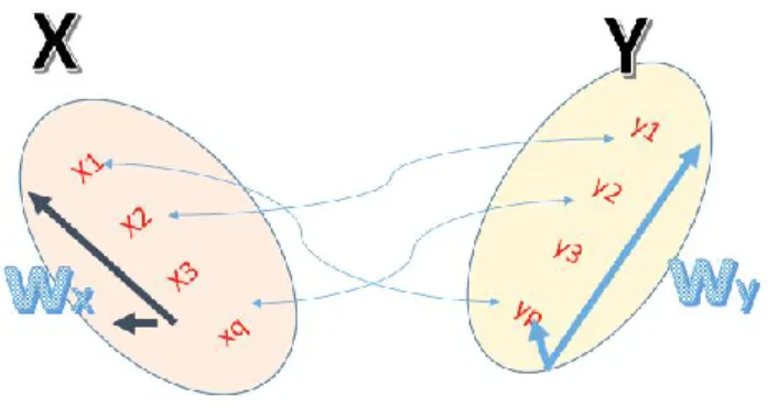
What is Canonical Correlation? Interrelationships between sets of multiple independent variables and multiple dependent measures quantify the strength of the relationship. Objectives of Canonical Correlation Analysis are to determine relationships among sets of variables, achieve maximal correlation, and explain the nature of relationships among sets of variables. Canonical correlation will be used to find linear/nonlinear combinations of both sets of variables Y and X that are maximally correlated. The objective in canonical correlation analysis is to determine simultaneous relationships between the two sets of variables. The canonical correlations between X and Y can be found by solving the eigenvalues equations (Konishi, 1979):
Where the eigenvalues 2 are the squared canonical correlations and the eigenvectors Wx and Wy
are the normalized canonical correlation basis vectors. The canonical eigenvectors summarize the correlation information between the X and Y variables.
Figure 1. Canonical Correlation Analysis Approach
Vectors Wx and Wy are called the canonical correlation vector, which are the transformation of the
48
1 yx yx
R , therefore, for two variables to be uncorrelated is equivalent that Ryx 1
In general, the determinant of the correlation matrix will equal 1.0 only if all correlations equal 0, otherwise the determinant will be less than 1. The determinant is related to the volume of the space occupied by the swarm of data points represented by standard scores on the measures involved. When the measures are uncorrelated, this space is a sphere with a volume of 1. When the measures are correlated, the space occupied becomes an ellipsoid whose volume is less than 1 (Konishi, 1979).
The ideal situation for canonical correlation to be most effective, in the sense of having smaller number of canonical vectors in order to reduce the dimensionality of our problem (consisting of q-variate vector Y & p-variate vector X), would be that the determinants for the dependent and independent have the following properties (Konishi, 1979):
1, 1
XX YY
R R
Namely, those components of vector Y (& vector X) are not highly correlated to each other. This assures the stability of the coefficients for vectors Wx and Wy. Specifically, for the reduction of
dimensionality, each of the components of vector Y should be highly correlated to components of vector X.
Given that RYX is not a square matrix, the usual definition of determinant of a matrix cannot be
applied. However, we can use the definition of non-square matrix determinant given by Radic
(1969), namely, let A= (aij) be an mXn matrix with m =< n. The determinant of A is defined as
1
1
1
1 1
1 ...
...
( 1) det ... ... ...
...
m
m
m
j j
r s j j n
mj mj
a a
A
a a
where 1, ... ; 1 2 ... ; 1 ...
m m
j j N r m s j j ,
As an example, for a rectangular matrix with 2 rows by 3 columns (2 by 3), namely A = [A1, A2,
A3] , its determinant is given by:
3 3 3
1 2 1 2 1 2
3 3 3
1 2 1 2 1 2
det a a a det a a det a a det a a
b b b
b b b b b b
As in the case of square matrices, the determinant of rectangular matrices represents the volume
generated by its column. Namely, every real m x n matrix A = [A1, ..., An] determines a polygon
in Rm (the columns of the matrix correspond to the vertices of the polygon) and vice versa. First
of all, the determinant of the rectangular matrix [A1, . . .,An ] is related to a volume of the
polyhedron (A1,..An). In general, the determinant of a m x (m +1) matrix [A1, . . . , Am+i] is
proportional with a volume of the orientated m-simplex (Ai . . . Am+1), as well (Sušanj & Radic,
1994):
1, 2,..., m1 ! 1, 2,..., m1
49
Radic (1969) showed if a row of A is identical to some other row or is a linear combination of other rows then |A| =0 and therefore the volume generated will be equal to zero, which is an indication of high collinear variables. In our case, the ideal situation for reduction of dimensionality is that (Stanimirović, 1997)
0
YX
Radic R , namely, that vectors Y and X are highly correlated.
In short, the conditions for stability of the canonical coefficient and the maximum reduction of dimensionality would be
1, 1, 0
XX YY YX
R R Radic R
In the appendix, a test to determine whether RXX 1,RYY 1is provided.
Time Series Approach with Canonical Correlation for Google Correlate
The concept of cross-correlation relates to the correlation of two time series or vectors Y and X at different points in time. As a simple example of cross-correlation, consider the problem of determining possible leading or lagging relations between two time series xt and yt.
If the modelyt Axt l wt holds, the series xt is said to lead yt for l > 0 and is said to lag yt for l <
0. This assumes that noise wt is uncorrelated with the xt series. Hence, the analysis of leading and
lagging relations might be important in predicting the value of yt from xt (Shumway, 2011).
In general, the vectors X and Y (or alternatively the canonical correlation vectors Wx & Wy) are
considered time dependent, namely
1 1
min( , ) min( , )
1 1
... , ... , , ... , ...
t t
t
q p t q p t
x y
t t
t Y x
qt pt y x
W W
y x
Y X or W W
y x W W
The Cross Correlation matrix can be defined as a function between vectors X(t) and Y(t) (or W(t)x
& W(t)y). The cross correlation function (CCF) is helpful for identifying lags of the x-variable that
might be useful predictors of yt. Namely, the values of the Wx-variable will be used to predict
future values of Wy. In the relationship between two time series (Wyt and Wxt), the series Wyt may
be related to past lags of the Wxt-series.
The cross correlation matrix for this canonical correlation problem is defined as
( ),
i t k i
W y W xt
CCF
where CCF is defined by:
( ) , 1 , t k n k
xt x y t k y t
Wy Wxt
Wyt Wxt
W W W W
50
Observe that the matrix takes into account only the cross correlation between the dependent and
independent canonical correlation variables Wyi and Wxi. For testing (Shumway, 2011) the cross
correlation function (CCF), have the following asymptotic approximation, namely, the large sample distribution of CCF(k), for k = 1, 2, . . . , K, where k is fixed but arbitrary, is normal with
mean zero and standard deviation
1 2
n if at least one of the processes is independent white noise.
Therefore, a simple test for the hypothesis of no cross-correlation,H0
y xt,t k 0,H0
y xt,t k 0 at = 5% is to whether the sample cross correlation ,
t t k
y x
r is included in confidence interval
,
2 2
t t k
y x
r
n n
to fail to reject 0
, 0t t k
y x
H or alternatively for the canonical correlation
analysis is:
( ),
2 2
t k
Wy Wxt
CCF
n n
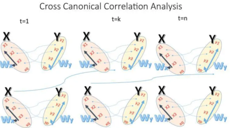
The CCF is the first step to create a predictive model taking into account the multiple correlations between vector X and Y. Combining the two approaches will obtain the following graphical summary:
Figure 2. Canonical Analysis with a Time Series Approach
Without loss of generality, consider the case vectors X and Y are highly related to each other and
within components of vectors X and Y have small correlations, namely
1, 1, 0
XX YY YX
R R Radic R ; then a small number of canonical correlation variables (Wx , Wy)
will explain the relationship between the X and Y vectors.
In the relationship between two time series (Wyt & Wxt), the series Wyt may be related to past lags
of the Wxt-series. Consider the first canonical correlation variables
1, , 1,
t t
X Y
W W with cross
correlation CCF k
, for k 0, 1, 2, . . . , KLet CCFmax be the largest of CCF(k) for a particular k*, which is significant at an level; then the
suggested model for the lagged relationship would be
*
1,Yt 1,Xt k t
W AW
. For example, if CCFmax
for k=1, then the correlation between 1,
t
Y
W is measured in time period t and
1
1,Xt
t-51
1, i.e. the correlation between 1,
t
Y
W is looked at in a time period and
1
1,Xt
W in the previous time
period.
In the case that RXX 0, RYY 0,Radic RYX 0, a similar approach can be used considering Principal Components Analysis (PCA) (Bilodeau & Brenner, 1999). PCA will be explained in a
following section below.
Collinearity, Canonical Correlation and Google Correlate
The case for RXX 0or RYY 0
Given the nature of Google Correlate, which finds queries highly related to each other, the
hypothesis to test RXX 1or RYY 1 may be rejected. In practice, Google Correlate may have
values supporting RXX 0or RYY 0. These correlation matrices for vectors Y and X may be
singular, i.e., the variables of vectors Y and X may be collinear.
A square matrix is singular if and only if its determinant is 0. This near singularity of the covariance matrix XXandYYwill create instability in the canonical vector coefficient,
In practice, XX andYYwill always have some degree of singularity. The researcher needs to determine his/her tolerance to correlation among the variables of vectors Y and X.
If RXX and RYY are close to 0, we can take advantage of this situation using firstly Principal component analysis (PCA) on the vectors Y and X, namely ZY= (Zy1, Zy2,…, Zyq) and ZX= (Zx1,
Zx2,…, Zxq) and then apply canonical correlation analysis, (Jolliffe, 2002). Principal component
analysis is simply an orthogonal transformation of the original Y into ZY and X into ZX.
Canonical correlations are invariant with respect to affine transformations of the variables. An affine transformation is simply a translation of the origin followed by a linear transformation. In mathematical terms an affine transformation of Rn is a map from Rn to Rn of the form (Borga,
2001):
( )
F p
Ap
q
for every vector p belonging to Rnwhere A is a linear transformation of Rn and q is a translation vector in Rn, therefore the application of principal components to the vectors Y and X will not alter the results of canonical correlation analysis.
Without loss of generalization, consider a simple bivariate problem with x1, x2 and y1, y2. A
52
performing the canonical correlation analysis on zx1, zx2 and zy1, zy2 separately rather than x1, x2
and y1, y2.
Also, zx1, zx2 and zy1, zy2 are exact linear functions of x1, x2 and y1, y2., respectively, and,
conversely, x1, x2 and y1, y2. are exact linear functions of , zx1, zx2 and zy1, zy2, respectively.
Consider the new equation for the q-variate Y and p-variate X whose values were transformed by Principal components ZY= (Zy1, Zy2,…, Zyq) and ZX= (Zx1, Zx2,…, Zxq), namely
By construction of the principal components, we have that
YY
Z
and
XX
Z
are diagonal matrices
and 1
XX YY
Z Z
R R
The number of principal components will be exactly q and p respectively, namely ZY= (Zy1,
Zy2,…, Zyq) and ZX= (Zx1, Zx2,…, Zxq). Some researchers may be tempted to drop some of the
principal components (the least informative ones) at this stage before performing canonical correlation analysis. In general, this is not advisable, as some Zxj may be dropped which are highly
related to Zyj. The researcher should use all principal components to perform the canonical
correlation analysis except when the number p and q are extremely large to reduce the dimensionality of the problem.
Similarly as in the previous section, the series Wzyt may be related to past lags of the Wzxt-series.
Consider the first canonical correlation variables
1, , 1,
t t
ZX ZY
W W with cross correlation
, 0, 1, 2, . . . ,CCF k for k K
Let CCFmax be the largest of CCF(k) for a particular k* which is significant at an level, then the
suggested model for the lagged relationship would be
*
1, t 1,
t k
ZY ZX t
W AW
.
In some situations like image processing and analysis, we may have p and q >> n, then a reduction technique such as PCA should be use to transform p and q to smaller set of variables with dimension p’ and q’ in such a way that p’ and q’ << n which could be attained. When p and q >> n and hypotheses RXX =1, RYY =1 is rejected, it is then advisable to perform PCA on p and q variables separately reducing number of variables to smaller set p’ and q’, then apply canonical
correlation analysis to these reduced number of principal components.
Application: Process Improvement with Google Correlate
53
queries with a similar pattern to a target data series. Let X and Y be vectors of words where it is assumed that X precedes Y, namely in the classical Google Correlate example of the flu, vector X can be fever, cough, weakness and vector Y can be flu, pneumonia, etc (Ginsberg, 2008).
Consider X(t) and Y(t) Google Correlate time dependent searches and Wyt and Wxttheir canonical
correlation counterparts. The cross correlation function will be used to determine the level of lag dependence between Wyt and Wxt to create a predictive model.
This methodology will be applied to the Toyota sudden acceleration problem. Since 1999, at least 2,262 Toyota and Lexus owners have reported to the National Highway Traffic Safety Administration, the media, the courts and to Safety Research & Strategies that their vehicles have accelerated suddenly and unexpectedly in a variety of scenarios. These incidents have resulted in 815 crashes, 341 injuries and, 19 deaths potentially related to sudden unintended acceleration. Figure 3 explains the order of Toyota acceleration and accident problems.
2006
Sept. National Highway Traffic Safety
Administration (NHTSA) opens
investigation on reports of “surging” in
Camrys: closes investigation a year later 2010
Jan. 21 Toyota recalls 2.3 million vehicles to correct separate problems that could cause gas pedal to stick Jan 26 Toyota suspends sales: halts production of eight models due to gas pedal recall; the next day. adds 1.1 million to floor mat recall
2007
March Toyota receives reports about accelerator pedal glitch in Tundra truck Sept. Toyota recalls some Lexus and Camry models to secure floor mat that could trap gas pedal, cause acceleration
Feb. 1 Toyota says it had developed fix for sticking gas pedal; begins shipping part to dealers
Feb. 3 NHTSA says it has received more than 100 complaints about brake problems in Prius hybrids
2008
Jan. NHTSA investigates unintended acceleration in Toyota Tacoma pickups: probe closed in Aug. after no detect found
Feb. 4 Toyota says gas pedal recall could cost $2 billion; total recall is 8.1 million; says Prius problem is software glitch; NHTSA opens Prius probe
2009
Aug. 28 Off-duty Calif. Highway Patrol officer, family killed after gas pedal in Lexus is caught under floor mat
Sep. 29 Toyota issues recall for 3.8 million vehicles due to risk of gas pedal becoming caught under floor mat Nov. 4 NHTSA accuses Toyota of providing
owners with “inaccurate and misleading information” about floor mat recall
Nov. 25 Toyota recalls at least 4 million vehicles to reconfigure gas pedals
Feb. 5 Toyota CEO makes first public appearance to apologize for recall problems
Feb. 9 437.000 Priuses recalled for brake problems: NHTSA says it has received complaints about steering problems in Corollas
Feb. 22 Federal prosecutors open criminal investigation into Toyota’s safety problems
Feb. 23 Congress begins hearings on Toyota recalls
Figure 3. Events related to Toyota accidents and Recall
The predictive model created helps to determine the number of lags (weeks) which could have
been used for the detection of Toyota Accidents.
Multivariate Approach using Canonical Correlations
54
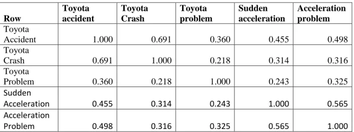
(Toyota accident, Toyota crash, Toyota problem) and vector X = (Sudden acceleration, Acceleration problem). The following Table 1 shows the correlation among the Y and X vectors which are significant at = 1%.
Table 1. Correlation among the Vector Y variables and Vector X variables
Row
Toyota accident
Toyota Crash
Toyota problem
Sudden acceleration
Acceleration problem
Toyota
Accident 1.000 0.691 0.360 0.455 0.498
Toyota
Crash 0.691 1.000 0.218 0.314 0.316
Toyota
Problem 0.360 0.218 1.000 0.243 0.325
Sudden
Acceleration 0.455 0.314 0.243 1.000 0.565
Acceleration
Problem 0.498 0.316 0.325 0.565 1.000
Let’s consider first the correlation between vector X and Y. The following table shows the
correlation among the Y and X vectors which are significant at family = 1%, (using a
Bonferroni adjustment).
Table 2. Correlation between dependent and independent variables
Row
Toyota accident
Toyota Crash
Toyota problem
Sudden
Acceleration 0.455 0.314 0.243
Acceleration
Problem 0.498 0.316 0.325
In matrix form, it will be:
0.455 0.314 0.243
0.498 0.316 0.325
R
In general, for the Radic determinant of R is given by
1, 1 1, 2 1, 3 11 12 13 11 12 11 13 12 13 2, 1 2, 2 2, 3 21 22 23 21 22 21 23 22 23 x y x y x y
XY
x y x y x y
Radic R
55
The first step for the canonical correlation analysis (CCA) if to check the appropriateness of CCA via Rao F= 21.769 (p-Value =0.000) with global R-square = 0.317 (Jolliffe, 2002)
The canonical correlation are given by
Canonical Coefficients for Dependent (y) Set
Table 3. Coefficient for the Canonical Vectors for Dependent and Independent Variables
Wy1 Wy2
Toyota accident ¦ 0.901 0.062 Toyota crash ¦ -0.050 -0.706 Toyota problem ¦ 0.276 0.860
Canonical Coefficients for Independent (x) Set
Wx1 Wx2
Sudden acceleration ¦ 0.435 -1.132 Acceleration problem ¦ 0.688 0.999
Based on the data of Table 3, as an example, the first canonical correlations are given by
1
1
0.901 0.50 0.276
0.435 0.688 y
x
W accident crash problem
W sudden acc problem
The correlation among the Canonical Correlation are given by
1, 1, 2, 2,
0.560
0.07
( , )
( , ) 2
y x y x
Corr W W
Corr W W
Let us consider the Cross Correlation analysis between the first two Canonical Correlations
1,y, 1,x
W W in order to develop a model such as
1,y 0 1 1, ,x t 1 2 1, ,x t 2 3 1, ,x t 3 ... 5 1, ,x t k* t
W W W W W
56
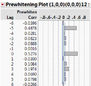
Figure 4. Cross Correlation Functions for the First Canonical Correlations for the dependent and Independent variables
Namely CCF W( 1, ,t y,W1,t5x)0.4878, which suggest the following model
W1,t(Y)=
b
0+b
1W1,t-5(X)and the graph showed in Figure 5.
Figure 5. Graphic representation of the cross correlation between the dependent and independent variables
Conclusions and Further Research
57
parameters to be considered and provides a useful framework to simplify the complexity of the problem. When the correlation among the component of vectors Y and X is not linear but monotonic the use of the Spearman correlation coefficient (nonparametric measure of rank correlation) is an alternative.
The following algorithm could be of use:
1. Select vector Yt and Xt time series from a database such as Google Correlation
2. Determine RXX 1,RYY 1; this is an indication that you can minimize the
number of variables contained in vector Y and X
3. Determine Radic RYX 0, namely vector Y and X are highly correlated; if this
condition is not fulfilled, stop and consider using VARMAX.
4. Apply Canonical Correlations to Model Y and X
5. Compute and test the canonical variables for Model Y and X namely Wy and Wx
6. Compute and test the Cross Correlation Function CCF(k*) for Wyt and Wxt
7. Based on 6) create a Time Series Regression Model
1,y 0 1 1, ,x t 1 2 1, ,x t 2 ... k* 1, ,x t k* t
W W W W
In 2) In Case of highly collinear vector Y or X , i.e., RXX 0,or R, YY 0, perform first Principal component Analysis.
For the case for Non-Linear Monotonic Correlation among the variables contained in
vectors Y and X, namely correlation between Y and X: Replace 1 by 1*
1. Select vector Yt and Xt time series from a database such as Google Correlation
and replace the values of vector Y and X by their ranks.
Replacing the values of Y and X by their ranks is equivalent to use the nonparametric correlation coefficients (such as the Spearman correlation coefficient) in RXX ,RYY ,Radic RYX .
References
Bilodeau, M., & Brenner, D. (1999). Theory of multivariate statistics. New York, NY: Spring Verlag.
Breusch, T., & Pagan, A. (1980). The lagrange lultiplier test and its applications to model specification in econometrics. The Review of Economic Studies, 47(1), 239-253.
Borga, M. (2001). Canonical correlation: A tutorial. Retrieved from: www.imt.liu.se/~magnus/cca/tutorial/tutorial.pdf
Chatfield, C. (2005). Time-series forecasting. New York, NY: Wiley Ed.
Stephens-Davidowitz, S., & Varian, H. (2015). A hands-on guide to Google data. Working paper. Google, Inc. Retrieved from:
58
Doornik, J. (1996). Testing vector error autocorrelation and heteroscedasticity. Proceedings of the Econometric Society 7th World Congress, Tokyo, Japan.
Ginsberg, J. (2008). Detecting influenza epidemics using search engine query data. Retrieved
from: http://research.google.com/archive/papers/detecting-influenza-epidemics.pdf
Granger, C. W. J., & Newbold, P. (1974). Spurious regression in econometrics. Journal of Econometrics, 2(2), 111-120.
Haig, B. (2006). Spurious correlation. Encyclopedia of measurement and statistics. Thousand
Oaks, CA: SAGE Publications.
Jolliffe, I. (2002). Principal component analysis (2nd ed.). New York, NY: Springer Verlag.
Konishi, S. (1979). Asymptotic expansions for the distributions of statistics based on the sample correlation matrix in principal component analysis. Hiroshima Math Journal, 9(3), 647-700.
Mohebbi, M., Vanderkam, D., Kodysh, J., Schonberger, R., Choi, H., & Kumar, S. (2011). Google
correlate whitepaper. Retrieved from: https://research.google.com/pubs/pub41695.html
Radic, M. (1969). A definition of the determinant of a rectangular matrix. Glasnik Matemaicki, 1, 1-21.
Preisendorfer, R. W., & Mobley, C. D. (1988). Principal component analysis in meteorology and oceanography (Vol. 17). Elsevier Science Ltd.
Quality Control Systems Corp (2011). Consumer complaints and warranty repairs in NASA-NHTSA’s Toyota study of unintended acceleration, July 21, 2011. Retrieved from
http://www.safetyresearch.net/Library/Report110721.pdf
Sušanj, R., & Radic, M. (1994). Geometrical meaning of one generalization of the determinant of square matrix. Glas Mat Ser, 29(2), 217-233.
Shumway, R. H., & Stoffer, D. S. (2010). Time series analysis and its applications: With R examples. New York, NY: Springer Science & Business Media.
Stanimirović, P., & Stanković, M. (1997). Determinants of rectangular matrices and Moore -Penrose inverse. Novi Sad Journal of Mathematics, 27(1), 53-69. Retrieved from
https://www.emis.de/journals/NSJOM/Papers/27_1/NSJOM_27_1_053_069.pdf
Tiao, G., & Tsay, R. (1989). Model specification in multivariate time series. Journal of the Royal Statistical Society, Series B (Methodological), 51(2), 157-213.
Author’s Biography
59
60
Appendix: Testing Independence for Vectors Y and X
In order to test RXX 1or RYY 1, more specifically
0 1
1
0
H Uncorrelated R
H Correlated R
we can use the Bartlett test, namely
2 ( 1)
2 2 5
1 ln
6
n
p p
p
n R
For any alternative degree of correlatedness or independence in the normal case other than R 1
or R 0
0 1
H R P
H R P
Konishi (1979) provides the following formula:
2 2
1 | | | | 0, 2 | | ( )
d