Forestry & Natural-Resource Sciences Last Correction: Sep. 9, 2013
COMPARING SPATIAL AND NON-SPATIAL APPROACHES FOR
PREDICTING FOREST SOIL ORGANIC CARBON AT
UNSAMPLED LOCATIONS
Brian J Clough, Edwin J Green
Center for Remote Sensing and Spatial Analysis, Department of Ecology, Evolution & Natural Resources Rutgers University, New Brunswick, NJ, USA
Abstract. Prediction of soil organic carbon (SOC) at unsampled locations is central to statistical modeling of regional SOC stocks. This is often accomplished by applying geostatistical techniques to plot
inventory data. However, in many cases inventory data is sparsely sampled (<0.1 plots/km2) relative to
the region of interest, and it is unknown if geostatistics provides any advantage. Our objective was to test whether modeling spatial autocorrelation, in multivariate and univariate predictive models, improved estimates of SOC at prediction locations based on sparsely-sampled inventory data. We conducted our study using a dataset sampled across all forested land in the Coastal Plain physiographic province of New Jersey, USA. We considered five models for predicting SOC, two linear regression models (intercept only and multiple regression with predictor variables), ordinary kriging (a univariate spatial approach), and two multivariate spatial methods (regression kriging and co-kriging). We conducted a simulation study in which we compared the predictive performance (in terms of root mean squared error) of all five models.
Our results suggest that our sparsely-sampled SOC data exhibits no spatial structure (Morans I=0.05,
p=0.39), though several of the covariates are spatially autocorrelated. Multiple linear regression had the
best performance in the simulation study, while co-kriging performed the worst. Our results suggest that when inventory data is dispersed across the region of interest, modeling spatial autocorrelation does not provide significant advantage for predicting SOC at unsampled locations. However, it is unknown whether this autocorrelation does not exist at broad scales, or if sparse sampling strategies are unable to detect
it. We conclude that in these situations, multiple regression provides a straightforward alternative to
predicting SOC for mapping studies, but that more work on the spatial structure of soil carbon across multiple scales is needed.
Keywords: Forest soil carbon; Geostatistics; Regression; Co-kriging; New Jersey; Coastal Plain.
1
Introduction
Globally, forests are thought to store approximately 861 petagrams of carbon (Pg C), with about 44% of this mass found in forest soils (Pan et al., 2011). The large capacity of the forest soil pool to sequester carbon makes its management a viable option for mitigating the effects of atmospheric carbon emissions (Goodale et al., 2002; Lal, 2008). Naturally, there is considerable in-terest in the quantification of forest soil organic carbon (SOC) pools for carbon monitoring projects and the de-velopment of market-based carbon accounting schemes. There is a need for methodologies that produce con-sistent results with a degree of accuracy acceptable to
policymakers (Chen et al., 2000a; Houghton, 2003; Shv-idenko et al., 2010).
Forest carbon stocks are typically measured using for-est inventories, and areal for-estimates are gained by “scal-ing up” these measurements across the region of interest (Birdsey, 1992; Goodale et al., 2002). However, these data are often sparse relative to the extent of the stock estimate. In the case of forests, soil carbon sampling is often excluded from large inventory efforts due to the additional time and cost needed to collect and process samples relative to aboveground forest measurements. As a result, regional estimates of forest soil carbon stor-age are often highly uncertain, leading to wide disparity among the literature. For example, estimates of carbon
stocks for European forest soils have ranged from 3 Pg C to as high as 79 Pg C; a difference that constitutes approximately 9% of the global forest soil carbon stock (Cannell et al., 1992; Goodale et al., 2002; Liski et al., 2002; Jones et al., 2005).
Developing a regional soil carbon stock from inven-tory data involves prediction of the response variable at many unsampled locations (i.e., all squares of a grid covering the region of interest). Spatial autocorrelation, where nearby points are on average more similar than points that are further apart, is a common property in environmental datasets and, when present in inventory data, may be leveraged to increase prediction accuracy (Simbahan et al., 2006). Spatial autocorrelation may be summarized by computing the semivariance, a mea-sure of spatial similarity, and plotting these values for all pair-wise combinations of the sampling points as a func-tion of distance (Goovaerts, 1997). These plots, typi-cally referred to as the empirical semivariogram, may be fitted with “theoretical” semivariogram models, such
as Mat´ern class or spherical functions. Kriging
meth-ods, a widely used class of spatial interpolators, incor-porate such theoretical semivariogram models to weight predictions at unsampled locations (Isaaks and Srivas-tava 1989). This feature, combined with the fact that these methods may be extended to model spatial co-variance between the response and predictor variables, makes kriging a logical approach for the prediction of soil carbon.
Geostatistical techniques have been successfully ap-plied to predict soil organic carbon at unsampled lo-cations, based on plot inventory data, at a variety of spatial scales. Several studies are available for
agricul-tural fields, where very dense sampling regimes (>400
plots/km2) can be achieved, and clear patterns of
spa-tial variation are often elucidated (Chen et al., 2000a; Lark, 2000; Mueller and Pierce, 2003; Simbahan et al.,
2006). In such situations, geostatistical models have
been shown to offer considerable improvement in pre-diction results when compared to non-spatial regression models (Simbahan et al., 2006).
Fewer examples are available for regional soil carbon mapping, where reduced sampling density may make
spatial autocorrelation more difficult to detect. Still,
several studies have shown an increase in prediction accuracy when incorporating geostatistical techniques. Liski and Westman (1997) used block kriging to interpo-late measurements of soil organic carbon taken as part of the national forest inventory (NFI) in Finland, and detected significant spatial structure in these clustered,
but densely sampled (∼5 plots/km2) data. More
re-cently Mishra et al. (2010) compared the performance of several geostatistical methods, including geographi-cally weighted regression and regression kriging, to
mul-tiple regression models for predicting SOC across a het-erogeneous region in the northern Midwestern United States. Their results suggest a significant increase in
prediction accuracy (∼22% relative improvement) when
incorporating spatial error into the model. Other ex-amples where significant spatial structure was detected and used to model SOC are available for grasslands in Ireland (McGrath and Zhang 2003, Zhang et al., 2011) and agricultural landscapes in the karst region of China (Liu et al., 2006; Zhang et al., 2012).
While the aforementioned studies modeled SOC across large spatial extents, most took advantage of
rea-sonably dense plot inventory data (≥0.1 plots/km2), and
in the case of Liski and Westman (1997) approximately
5 plots/km2. The exception is the study by Mishra et
al. (2010), which utilized sparsely sampled data (∼0.003
plots/km2), but modeled SOC across a heterogeneous
landscape with several major cover types and a pro-nounced latitudinal gradient (from the upper Peninsula of Michigan south to Kentucky, USA), both of which may exert strong controls on SOC distribution. When the region of interest comprises a single cover class, as it would in forestry applications, or does not span many degrees of latitude, it is less clear that modeling spa-tial autocorrelation presents any advantage for predict-ing forest SOC. In fact, a few studies provide evidence suggesting this is the case. Studies in tropical forests that examined forest SOC across multiple scales, in trop-ical dry forests in the West Indies (Gonzalez and Zak, 1994) and in the Brazilian Amazon (Cerri et al., 2000; Bernoux et al., 2006), suggest that the spatial structure is limited to fine scales only.
In this study, our primary objective was to assess whether incorporating spatial autocorrelation into mod-els for predicting forest soil organic carbon at unsampled
locations improved results for sparsely sampled (<0.1
plots/km2) inventory data. To meet our objective, we
compared the performance of both univariate and mul-tivariate spatial models to similar linear regression mod-els. We predicted that the spatial models would perform the best when predicting forest SOC at independent val-idation locations, despite the sparsity of our sampling locations relative to the region of interest. To test this prediction, we developed a simple simulation experiment to directly compare the predictive accuracy of all models considered in the experiment.
2
Methods
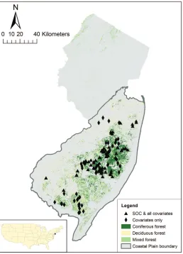
2.1 Study region This study was conducted on the Coastal Plain physiographic province of New Jersey,
USA (Fig. 1). This region is largely forested, and
for-Figure 1: Distribution of sampling locations and primary forest cover types across the study region in New Jersey, USA.
est communities dominate the region: (1) pitch pine (Pinus rigida) forest, (2) oak (Quercus spp.) forest, and (3) mixed communities that span a gradient be-tween these two classes (Hasse and Lathrop, 2010). On the inner coastal plain, these communities mix with
other hardwood species such as American beech (
Fa-gus grandifolia) and hickory (Carya) spp. Forested wetlands are common along river courses or in low
ar-eas. Most of these are hardwood swamps dominated
by red maple (Acer rubrum), sweetgum (Liquidambar
styraciflua), and blackgum (Nyssa sylvatica). However, forested peat bogs with pure stands of Atlantic white
cedar (Chamaecyparis thyoides) are also present across
the landscape. Soils in the region are largely typic Hap-ludults and Quartzisappamments of marine or alluvial origin (Tedrow, 1986). Soils range from very poorly to excessively drained, and are primarily sandy in texture. However, clayey and mucky soils are frequent in wet ar-eas. The total area of the study region (i.e., all forested land in New Jersey’s Coastal Plain) is approximately
4,522 km2.
car-bon and all of the covariates used in the model ex-periments. This corresponds to a sampling density of
approximately 0.013 plots/km2. The “large” dataset
consists of 120 plots and contains measurements of the model covariates only, and was used for the co-kriging
analysis. The small dataset is a subset of the large
dataset, so those 62 plots are co-located and present in each. The plots were sampled in a stratified random design across the landscape, based on both forest com-munity type and soil drainage class (Fig. 1).
At each sampling location, soil was collected from three depth intervals: 0-10 cm, 10-20 cm, and 20-30 cm. At each depth interval bulk density was sampled using the core method (Blake and Hartge, 1986), and a second sample was taken for laboratory analysis. Bulk
density samples were dried for 24 hours at 105 ◦C and
passed through a 2 mm sieve to remove the coarse frag-ments (i.e., gravel and litter material) that are not a component of the soil organic matter pool. The analyt-ical samples were air dried for at least 48 hours, sieved to 2 mm, then ground into powder with a mortar and pestle and homogenized.
Percent soil organic carbon was estimated by elemen-tal (CHN) analysis on a subsample of the air-dried ana-lytical sample. A second subsample was used to measure percent soil organic matter (SOM) by loss-on-ignition (LOI). These data were recorded for all 120 plots, and used as a covariate in the multivariate models. SOM typ-ically has a significant relationship with SOC, and has been used as a predictor for soil organic carbon in several studies (Konen et al., 2002; De Vos et al., 2005). Sam-ples were placed in a Lindberg muffle furnace (General
Signal, Watertown, WI, USA) at 400 ◦C for 24 hours.
Both percent SOC and percent SOM were converted to stock estimates using the following formula:
S=P×BD×V ×g (1)
where S is the stock estimate (Mg·ha−1), P is a percent
measurement of SOC or SOM, BD is soil bulk density
(g·cm−3), V is the volume of a 1 ha rectangle with a
depth of 30 cm, and g is a unit scaling constant.
2.3 Model covariates In addition to the plot mea-sured soil organic matter data, we utilized four covari-ates extracted from remote sensing and GIS datasets: normalized difference vegetation index (NDVI), band 2 of the “tasseled cap” transform (TC2), compound to-pographic index (CTI), and elevation (ELEV). These variables represent a reasonable set of potential predic-tors for soil organic carbon, and are similar to covariates incorporated by several recent regional SOC mapping studies (McGrath and Zhang, 2003; Mishra et al., 2010; Vasques et al., 2012; Zhang et al., 2012). NDVI and TC2, the “greenness” band of the tasseled cap
trans-form, are both related to net photosynthetic output, which has a theoretical relationship to inputs into the soil organic carbon pool (Chapin et al., 2002). Terrain position can have a strong influence on soil organic car-bon storage, so we included two related variables: eleva-tion and estimates of the compound topographic index (CTI). CTI is a steady state wetness index designed to model soil water content based on values of slope and flow direction extracted from a digital elevation model (Moore et al., 1991). It has been shown to correlate with soil moisture content, which may exert influence over soil organic carbon formation and storage (Barling et al., 1994).
To extract the NDVI and TC2 measurements for our sampling locations, cloud-free Landsat TM scenes (http://glovis.usgs.gov) were downloaded for a single
date during the study, July 14th 2011, and tiled into a
mosaic of the study region. We used a Level 1 data prod-uct from the Landsat 5 thematic mapper instrument that had been previously corrected for radiometric error and terrain variability, geo-referenced, and converted to Universal Transverse Mercator (UTM) projection. The Erdas Imagine software package (Leica Geosystems, At-lanta, GA, USA) and ArcGIS (ESRI, Redlands, CA) were used to separately generate rasters for both vari-ables with a 30-m x 30-m grid cell size for all forested land within the study region, and to extract values of NDVI and TC2 for our sampling locations. Both the elevation and CTI data were derived from a 10-m dig-ital elevation model (DEM) provided by the Center of Remote Sensing and Spatial Analysis (CRSSA), Rut-gers University. Compound topographic index was cal-culated for all cells in the DEM using ArcGIS.
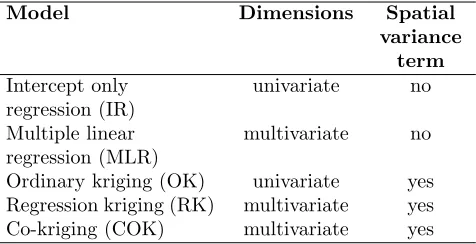
2.4 Modeling approaches Our objective in this study was to test whether explicitly modeling spatial autocorrelation improved prediction accuracy for our sparsely sampled forest SOC data. To accomplish this we considered five models that represent spatial and non-spatial approaches for both univariate (SOC data only) and multivariate (incorporating the predictor variables) cases (Tab. 1). This design allowed us to both examine the effect of modeling spatial autocorrelation only, in the case of the univariate spatial model (OK), as well as the influence of the spatial variance term for two different multivariate approaches.
Our non-spatial approach was linear regression models (MLR) of the general form:
Y = α+ βj∗X (2)
WhereY is soil organic carbon,X is ann x p matrix
of the predictor variables, αis the intercept, andβj is
Table 1: Dimensions and spatial variance assumptions for the five predictive models considered in this study.
Model Dimensions Spatial variance
term
Intercept only regression (IR)
univariate no
Multiple linear regression (MLR)
multivariate no
Ordinary kriging (OK) univariate yes
Regression kriging (RK) multivariate yes
Co-kriging (COK) multivariate yes
covariate. In the case of the intercept only model (IR),
αis the only parameter.
All three of the spatial models we incorporated are variations on the kriging algorithm, where spatial pre-diction is accomplished as a function of the theoretical semivariogram; a model fitted to a plot of semivariance values against distance for each pair-wise combination of sampling locations in the dataset (i.e., the empirical variogram) (Goovaerts 1997). For the univariate model (OK), the linear estimator used to predict new values of
the response variable, for some set of locationsu, takes
the form:
Z∗(u) =m(u) + n(u) X
α=1
λα(u) [(Z(uα)−m(u)] (3)
WhereZ*(u)is the predicted value of the response
vari-able at new locations, Z(uα) are the known values of
the response at sampled locations,m(u) is the mean
re-sponse, and theλα’s are the “kriging weights” for each
sampled location, that are determined by the
semivari-ogram model (Goovaerts, 1997; Simbahan et al., 2006).
In the case of ordinary kriging, note that the mean is
taken to be a function of the locations u so that it is
allowed to vary across the region (Isaaks and Srivastava, 1989).
In addition to the univariate OK model, we consid-ered two different approaches for incorporating covari-ates into spatial models. The first of these is regression kriging (RK), which is very similar to OK in principle. The difference is that the residuals of the response and predictor variables are interpolated, and in this way co-varying spatial patterns are indirectly incorporated into the analysis (Odeh et al., 1994; Hengl et al., 2004; Sim-bahan et al., 2006). For prediction at new locations, the spatially predicted residuals must be added back on to the mean trend, resulting in the following linear
estima-tor forZ∗(u):
Z∗(u) = p
X
k=0
βkqk(u) + n(u) X
α=1
λαe(u) (4)
Whereβk are the regression parameters associated with
the predictors qk, p is the number of predictors, and
e(u)are the residuals between the response and
covari-ables (Hengl et al., 2003, 2004). The rest of the terms in the model are as defined above. We wish to note that the technique we outline here is one of several closely related approaches that have all variously been termed “regression kriging”, “kriging with external drift”, and “kriging with a trend” (Goovaerts, 1997; Wackernagel, 1998; Chiles and Delfiner, 1999). We follow Hengl et al. (2004) in describing the method outlined above, where fitting the non-spatial trend and the spatial interpolation of the residuals are accomplished separately, as regres-sion kriging.
The second multivariate method considered here is co-kriging (COK), which represents a particularly flex-ible approach to modeling multivariate geostatistical data. Rather than interpolating residuals between the response and predictor variables, COK starts with the fitting of both direct and cross variograms for all vari-ables in the model, typically with a linear model of core-gionalization (Gelfand et al., 2004). This variogram sys-tem is employed to weight predictions of the response variable at new locations, according to the following lin-ear estimator:
Z∗(u) = m(u) + n1(u)
X
α1=1
λα1(u) [Z1(uα1)−m1(uα1)]
+ Nv X
i=2
ni(u) X
αi=1
λαi(u) [Zi(uαi)−mi(uαi)] (5)
WhereZ*(u)is the predicted value of the response
vari-able at new locations,λα1is the weight assigned to the
re-sponse variableZ1andλαirepresents the weights for the
covariates Zi(Goovaerts, 1997; Simbahan et al., 2006).
In this model, the expected values mi are subtracted
from the data, indicating we consider the spatial asso-ciation between the response and predictor variables to be a multivariate stationary process.
response variable. This situation lends itself well to the co-kriging approach.
2.5 Model comparison simulation To compare the performance of the five models for predicting soil or-ganic carbon, we devised a simulation that compared predicted vs. actual results for independent validation data. We first randomly divided the “small” dataset into fitting and validation datasets. We reserved 25% of the data for validation (N=15) and reserved the re-maining 47 plots to fit the models. We split the data this way, rather than using an even split, because ini-tial runs of several kriging models resulted in undefined covariance functions when N=31 for the model fitting data. A fitting set of 47 plots translates to a density of
approximately 0.01 plots/km2 across the study region.
In the case of the COK model, the additional covariate observations in the “large” dataset were included in the model fitting, as the structure of the coregionalization model permits this design. To increase normality, all variables were log-transformed prior to fitting the mod-els. Each model was used to predict SOC for the valida-tion dataset, and we computed root mean squared error (RMSE) to assess model performance. Prior to com-puting RMSE, predicted values of log(SOC) were back-transformed into their original units. To avoid biasing results by selecting a single, favorable fitting dataset we ran this simulation for 10,000 iterations and tracked mean RMSE for the entire study. This is especially rel-evant for the geostatistical models, as relatively sparse datasets such as ours may possess spatial autocorrela-tion with some configuraautocorrela-tions but not with others.
To initialize the OK and COK models, we supplied values for the sill, range, and nugget parameters
de-rived by fitting a Mat´ern class covariance function to the
empirical variograms for soil organic carbon in the full dataset. In the co-kriging model, these values were used to initialize the parameters for all direct and cross vari-ograms. In the case of RK, we supplied initial parameter values from a theoretical variogram fitted to the residu-als of SOC and the model covariates. All model fitting
was accomplished with ordinary least squares. A Mat´ern
covariance function was selected because it is a particu-larly flexible model for spatial autocorrelation, and is a popular choice in current geostatistical research (Stein, 1999; Finley et al., 2011). The simulation was conducted using the R statistical computing environment. Vari-ogram fitting, OK, and RK were conducted using the geoR package (Ribeiro and Diggle, 2001), and co-kriging was accomplished in the gstat package (Pebesma, 2004).
Table 2: Mean (µ), standard deviation (σ2), and slope
parameters (βj) and correlation coefficients (ρ) for the
five covariates and SOC.
µ σ2 βj ρ
SOC (Mg·ha−1) 65.93 65.67 ** **
SOM (Mg·ha−1) 113.17 153.66 0.678 0.708
NDVI 0.61 0.05 0.395 0.103
TC2 29.54 9.13 -0.507 0.046
CTI 9.99 2.48 0.332 0.106
ELEV (m) 26.35 12.25 0.157 0.098
3
Results
3.1 Exploratory analysis Table 2 presents the mean and standard deviation for all variables, as well as the regression parameters for the MLR model and the correlation coefficients between log(SOC) and each of the covariates for the full dataset (N=62). Soil
or-ganic matter is highly correlated with SOC (ρ=0.708),
while the remaining variables are not notably correlated (ρ<0.2 for each). For the intercept only model, α = 3.59.
Examination of the spatial structure in the SOC dataset does not reveal any spatial autocorrelation
among the 62 sample sites (Moran’s I=-0.05, p=0.39).
However, slight positive spatial autocorrelation was
noted for the following covariates: TC2 (Moran’s
I=0.06, p=0.04), CTI (Moran’s I=0.05, p=0.09), and
ELEV (Moran’s I=0.036, p<0.001). Both SOM and
NDVI do not possess significant spatial autocorrelation
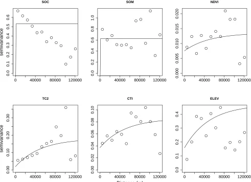
(p>0.10). The empirical variograms, as well as the
fit-ted Mat´ern covariance functions (i.e., the theoretical
variograms), agree with these results (Fig. 2). TC2, CTI, and ELEV show an increase in semivariance across
distance, each with an asymptotic range > 120,000 m.
However, note that there is considerable residual error between the empirical semivariance values and the fitted covariance model. NDVI suggests an increase in semi-variance, but the scale of the y-axis for this plot indicates a minute change across the effective range. Both SOC and SOM do not show spatial structure in either the empirical or theoretical semivariograms.
0 40000 80000 120000
0.0
0.1
0.2
0.3
0.4
0.5
0.6
SOC
semiv
ar
iance
0 40000 80000 120000
0.0
0.2
0.4
0.6
0.8
1.0
SOM
0 40000 80000 120000
0.000
0.005
0.010
0.015
0.020
NDVI
0 40000 80000 120000
0.00
0.10
0.20
0.30
TC2
semiv
ar
iance
0 40000 80000 120000
0.00
0.02
0.04
0.06
0.08
0.10
CTI
Distance (m)
0 40000 80000 120000
0.0
0.1
0.2
0.3
0.4
ELEV
Figure 2: Empirical (open circles) and theoretical (solid lines) variograms for the response (SOC) and the five covariates.
of MLR. Comparing the two univariate methods also suggests a disadvantage to modeling spatial autocorre-lation, as the IR model reduced error when compared to the OK model.
4
Discussion
In contrast to studies where prediction of SOC is
ac-complished with relatively dense plot inventories (>0.1
plots/km2) (e.g., Liski and Westman, 1997; Lark, 2000;
McGrath and Zhang, 2003; Simbahan et al., 2006; Zhang et al,. 2012), we found that modeling spatial autocorre-lation did not improve prediction accuracy at unsampled locations for our sparse inventory data. Both variogram
analysis and Moran’s I statistics suggest a lack of
tial autocorrelation in our soil carbon data. While spa-tial structure was noted in some of the covariates, the lack of spatial structure in SOC resulted in inferior per-formance of the spatial models relative to MLR. How-ever, note that the RMSE of all models is large relative
Table 3: Results of the simulation experiment. Note that this table presents back-transformed values of for-est SOC. Mean RMSE refers to the mean root mean squared error over the 10,000 trials in the simulation experiment. RI refers to the relative improvement in predictive performance of each model, when compared to the worst performing method (Ordinary Kriging).
Model Mean
RMSE (Mg·ha−1)
RI
(%)
Intercept only regression (IR) 59.65 12.1
Multiple regression (MLR) 51.52 24.1
Ordinary kriging (OK) 67.9 –
Regression kriging (RK) 53.43 21.3
to the mean of soil carbon for the whole dataset (65.9
Mg·ha−1), suggesting that there is a high degree of
un-certainty in all five models.
Generally, these results highlight the difficulties of spatial prediction of forest soil carbon. A number of studies have identified spatial structure at local scales in a variety of forest types, with variogram range param-eters from 4-500 mparam-eters (e.g., Robertson et al., 1993; Lister et al., 2000; Wang et al., 2002; Garten Jr. et al., 2007; Worsham et al., 2010). It is not known, however, if these fine-scale spatial dynamics are meaningful to pre-dictions for regional datasets, where distances between plots may range from one to hundreds of kilometers. Further, it remains unclear whether spatial autocorre-lation at broad scales is an important factor in under-standing regional forest carbon dynamics. Our results suggest otherwise, as do those of the few other studies that have looked at this question (Liski and Westman, 1997; Cerri et al., 2000; Bernoux et al., 2006).
In our data, determining whether regional forest SOC data truly exhibits no spatial structure, or if this is the result of a detectability issue caused by low sampling densities, remains unclear. Assuming spatial structure exists at the regional scale, describing it may require a large number of observations relative to the region of interest. While national forest inventories, such as the US Forest Service’s Forest Inventory and Analysis (FIA) program, may achieve the requisite densities for above-ground measurements (Finley et al., 2007), collection of data on soil variables is often only completed at a fraction of these plots. Further, the ability to detect spatial autocorrelation is influenced by the sampling de-sign (Fortin et al., 1989). Thus, surveys may need to be specifically designed to detect broad-scale spatial struc-ture in forest soils.
Those studies which have detected regional spatial autocorrelation in the soil organic pool have typically done so over heterogeneous landscapes, spanning mul-tiple cover classes (McGrath and Zhang, 2003; Mishra et al., 2010; Vasques et al., 2010; Zhang et al., 2011). In these contexts, the spatial structure of soil carbon is influenced by other spatially-explicit dynamics, such as patterns in land use and land cover, which may make regional patterns easier to define (Vasques et al., 2012). Modeling soil carbon over very large regions, such as the northern portion of the Midwestern United States (Mishra et al., 2010), also incorporates the effect of lat-itudinal climate gradients which are well known to
in-fluence soil organic carbon (Chapin et al., 2002). In
this way, Mishra et al. detected an advantage to spatial approaches (geographically weighted regression and re-gression kriging) over multiple rere-gression despite a very
low plot density (<0.001 plots/km2). In forestry
appli-cations, particularly across comparatively small regions
such as the Coastal Plain of New Jersey, there may be fewer influences on the regional spatial structure of soil organic carbon. However, additional studies in different forest types will be necessary to determine if this is in fact the case.
Incorporating covariates of soil carbon into predictive models is a typical strategy, and one employed by al-most all of the studies outlined here. In our case, four of the five covariates we considered were not strongly cor-related with forest SOC. These patterns may be unique to our region in some ways. For instance, one would expect a strong relationship between soil organic carbon and elevation. However, the Coastal Plain of New Jersey is a fairly low-relief landscape, and fully capturing the covariance between SOC and elevation in an inventory dataset may be particularly challenging.
Field measured soil organic matter was the one covari-ate that was reasonably correlcovari-ated with SOC, but given that this variable was also sampled as part of our for-est inventory it has limited usefulness for predicting soil carbon at unsampled locations. For regression models, it is generally necessary to have values for the covari-ates at the prediction locations (i.e., for all cells of a sampling grid in mapping applications). Methods based on fitting coregionalization models, such as co-kriging, are attractive in that they do not share this prerequi-site (Goovaerts, 1997; Banerjee et al., 2004; Gelfand et al., 2004). However, in the absence of spatial structure in the response variable, these methods will likely yield poor results, as was the case with our data. An alter-native strategy is to model the spatial dynamics of the covariates themselves. For example, soil organic matter may be interpolated based on ancillary variables in order to inform a sampling grid for soil carbon. However, this introduces additional sources of uncertainty which may propagate through to the final estimate of the response variable.
The results of our study have applications for forest SOC mapping projects, particularly where new inven-tories are being established to accomplish these goals. This may be especially relevant in developing coun-tries, where international funding mechanisms such as the United Nations’ Reducing Emissions from Deforesta-tion and DegradaDeforesta-tion (REDD+) program has motivated increased interest in managing forests to offset carbon emissions (Edwards et al., 2010). Newly established for-est inventories will be important for both gathering base-line data on forest carbon stocks in these regions, and for verifying gains in carbon sequestration (Maniatis and Mollicone, 2010). Our results suggest that when plot
inventories are sparsely distributed (<0.1 plots/km2),
multiple linear regression presents a straightforward al-ternative, providing a set of reasonable covariates can be identified for all prediction locations.
Taken in context with the existing literature on the spatial dynamics of forest SOC, our work highlights the need for more studies that explicitly model soil carbon across a range of spatial scales. Without these data, it remains unknown whether regional spatial autocorre-lation does not exist or requires more dense sampling schemes to detect. Further, our results are from but one forest type, and it is not clear that the dynamics we describe are generalizable to other forest ecosystems. That all of our models provide a fairly poor fit to our SOC data demonstrates just how challenging character-izing uncertainty in regional soil carbon stocks can be. Advanced statistical modeling techniques such as geo-statistics present many appealing methods for the pre-diction of forest soil carbon, but their utility is premised on a set of assumptions that the available data may not meet. We advocate that these methods are considered for the prediction of forest carbon, and for SOC map-ping studies, but only when their use is warranted by the data.
5
Conclusions
When predicting soil organic carbon at unsampled lo-cations based on sparse inventory datasets, it may be dif-ficult to detect a significant degree of spatial autocorrela-tion. This is especially true on homogeneous landscapes, or for studies that only consider one cover type, as there may be spatial structure associated with the correlation between SOC density and land cover type. In such cases, geostatistical models may be inappropriate, and multiple linear regression offers an appealing and straightforward alternative. Including covariates can increase the tive performance of statistical models. The best predic-tors will not only be closely correlated with soil organic carbon, but will be available for the full extent of the study region. The results of our study have implications for SOC mapping approaches using existing inventories, where analytical efforts are constrained by data qual-ity and availabilqual-ity, as well as for new sampling efforts where resources are limited. Future work should look to model spatial autocorrelation of soil carbon across multiple scales, to fully characterize the relationship of well-described local spatial structure to broad-scale, re-gional patterns.
Acknowledgements
We thank the guest editors and the three anonymous reviewers for their helpful comments. Additionally, we wish to acknowledge the funding we have received from
the United States Forest Service and Rutgers, The State University of New Jersey.
References
Banerjee, S., B. P. Carlin, and A. E. Gelfand. 2004. Hierarchical Modeling and Analysis for Spatial Data. Chapman & Hall, Boca Raton, FL. 472 p.
Barling, R., I. D. Moore, and R. B. Grayson. 1994. A quasi-dynamic wetness index for characterizing the spatial distribution of zones of surface saturation and soil water content. Water Resour. Res. 30:1029-1044.
Bernoux, M., D. Arrouays, C. E., P. Cerri, and C. C. Cerri. 2006. Regional organic carbon storage maps of the western Brazilian Amazon based on prior soil maps and geostatistical interpolation. Dev. Soil Sci. 31:497-506.
Birdsey, R. A. 1992. Carbon storage and accumulation in United States forest ecosystems. USDA For. Serv. Gen. Tech. Rep. WO-59. 55 p.
Blake, G. R., and K. H. Hartge. 1986. Bulk Density. P.377-382 in Methods of Soil Analysis Part 1. Physi-cal and MineralogiPhysi-cal Methods, A. Klute (ed.). Amer-ican Society of Agronomy, Inc.; Soil Science Society of America Inc., Madison, WI, USA.
Cannell, M. G. R., R. C. Dewar, and J. H. M. Thornley. 1992. Carbon flux and storage in European forest. P. 256-271 in Responses of Forest Ecosystems to Envi-ronmental Changes, A. Teller, P. Mathy, and J. N. R. Jeffers (eds.). Elsevier, London.
Cerri, C. C., M. Bernoux, D. Arrouays, B. J. Feigl, and M. C. Piccolo. 2000. Carbon Stocks in Soils of the Brazilian Amazon. in Global climate change and trop-ical ecosystems, R. Lal, M. Kimble, and B. A. Stewart (eds.). CRC Press, Boca Raton, FL.
Chapin, F. S., P. A. Matson, and H. A. Mooney. 2002. Principles of terrestrial ecosystem ecology. Springer Science & Business Media Inc., New York, NY. 350 p.
Chen, F., D. E. Kissel, L. T. West, and W. Adkins. 2000a. Field-scale mapping of surface soil organic car-bon using remotely sensed imagery. Soil Sci. Soc. Am. J. 64:746-753.
Chen, W., J. Chen, J. Liu, and J. Cihlar. 2000b. Ap-proaches for reducing uncertainties in regional forest carbon balance. Global Biogeochem. Cycles 14:827-838.
De Vos, B., B. Vandecasteele, J. Deckers, and B. Muys. 2005. Capability of loss-on-ignition as a predictor of total organic carbon in non-calcaerous forest soils. Commun. Soil Sci. Plant Analysis 36:2899-2921.
Edwards, D. P., B. Fisher, and E. Boyd. 2010. Protecting degraded rainforests: enhancement of forest carbon stocks under REDD+. Conserv. Letters 3:313-316.
Finley, A. O., S. Banerjee, and R. E. McRoberts. 2007. A Bayesian approach to multi-source forest area esti-mation. Environ. Ecol. Stat. 15:241-258.
Finley, A. O., S. Banerjee, and D. W. Macfarlane. 2011. A hierarchical model for quantifying forest variables over large heterogeneous landscapes with uncertain forest areas. J. Am. Stat. Assoc. 106:31-48.
Fortin, M.J., P. Drapeau, and P. Legendre. 1989. Spatial autocorrelation and sampling design in plant ecology. Vegetatio. 83:209-222.
Garten J., C. T., S. Kang, D. J. Brice, C. W. Schadt, and J. Zhou. 2007. Variability in soil properties at different spatial scales (1m-1km) in a deciduous forest ecosystem. Soil Biol. Biochem. 39:2621-2627.
Gelfand, A. E., A. M. Schmidt, S. Banerjee, and C. F. Sirmans. 2004. Nonstationary Multivariate Process Modeling Through Spatially Varying Coregionaliza-tion. Test. 13:263-312.
Gonzalez, O. J., and D. R. Zak. 1994. Geostatistical analysis of soil properties in a secondary tropical dry forest, St. Lucia, West Indies. Plant and Soil. 163:45-54.
Goodale, C. L., M. J. Apps, R. A. Birdsey, C. B. Field, L. S. Heath, R. A. Houghton, J. C. Jenkins, et al. 2002. Forest Carbon Sinks in the Northern Hemi-sphere. Ecol. App. 12:891-899.
Goovaerts, P. 1997. Geostatistics for Natural Resources Evaluation. Oxford University Press, New York. 496 p.
Hasse, J. E., and R. G. Lathrop. 2010. Changing Land-scapes in the Garden State: Urban Growth and Open Space Loss in NJ 1986 thru 2007. Center for Remote Sensing and Spatial Analysis, Rutgers University, New Brunswick, NJ, USA.
Hengl, T., G. Heuvelink, and A. Stein. 2003. Com-parison of kriging with external drift and regression kriging. Technical Report, International Institute for Geo-Information Science and Earth Observation, En-schede. 18 p.
Hengl, T., G. Heuvelink, and A. Stein. 2004. A generic framework for spatial prediction of soil variables based on regression-kriging. Geoderma 120:75-93.
Houghton, R. a. 2003. Why are estimates of the terres-trial carbon balance so different? Glob. Change Biol. 9:500-509.
Isaaks, E. H., and M. Srivastava. 1989. An Introduction to Applied Geostatistics. Oxford University Press, Ox-ford. 592 p.
Jones, R. J. A., R. Hiederer, E. Rusco, P. J. Loveland, and L. Montanarella. 2005. Estimating soil organic carbon in the soils of Europe for policy support. Eur. J. Soil Sci. 56:655-671.
Konen, M. E., P. M. Jacobs, C. L. Burras, B. J. Talaga, and J. A. Mason. 2002. Equations for predicting soil organic carbon using loss-on-ignition for North Cen-tral U.S. soils. Soil Sci. Am. J. 66:1878-1881.
Lal, R. 2008. Carbon sequestration. Philos. T. Roy. B. 363:815-30.
Lark, R. M. 2000. Regression analysis with spatially au-tocorrelated error: simulation studies and application to mapping of soil organic matter. J. Geogr. Info. Sci. 14:247-264.
Liski, J., and C. J. Westman. 1997. Carbon storage in forest soil of Finland. Biogeochemistry 36:261-274.
Liski, J., D. Perruchoud, and T. Karjalainen. 2002. In-creasing carbon stocks in the forest soils of western Europe. Forest Ecol. Manag. 169:159-175.
Lister, A. J., P. P. Mou, R. H. Jones, and R. J. Mitchell. 2000. Spatial patterns of soil and vegetation in a 40-year-old slash pine (Pinus elliottii) forest in the Coastal Plain of South Carolina, U.S.A. Can. J. For. Res. 30:145-155.
Liu, D., Z. Wang, B. Zhang, K. Song, X. Li, J. Li, F. Li, and H. Duan. 2006. Spatial distribution of soil or-ganic carbon and analysis of related factors in crop-lands of the black soil region, Northeast China. Agric., Ecosyst. Environ. 113:73-81.
Maniatis, D., and D. Mollicone. 2010. Options for sam-pling and stratification for national forest inventories to implement REDD+ under the UNFCC. Carbon Balance Manage. 5:9-16.
Mishra, U., R. Lal, D. Liu, and M. Van Meirvenne. 2010. Predicting the Spatial Variation of the Soil Organic Carbon Pool at a Regional Scale. Soil Sci. Am. J. 74:906.
Moore, I. D., R. B. Grayson, and A. R. Ladson. 1991. Digital terrain modelling: a review of hydrological, geomorphological, and biological applications. Hydrol. Process. 5:3-30.
Mueller, T. G., and F. J. Pierce. 2003. Soil Carbon Maps: Enhancing Spatial Estimates with Simple Ter-rain Attributes at Multiple Scales. Soil Sci. Soc. Am. J. 67:258–267.
Odeh, I., A. McBratney, and D. Chittleborough.
1994. Further results on prediction of soil properties from terrain attributes: heterotropic cokriging and regression-kriging. Geoderma. 63:197-214.
Pan, Y., R. A. Birdsey, J. Fang, R. A. Houghton, P. E. Kauppi, W. A. Kurz, O. L. Phillips, et al. 2011. A large and persistent carbon sink in the world’s forests. Science 333:988-993.
Pebesma, E. J. 2004. Multivariable geostatistics in S: the gstat package. Comput. Geosci. 30:683-691.
Ribeiro, P. J., and P. J. Diggle. 2001. geoR: a package for geostatistical analysis. R-NEWS. 1:15-18.
Robertson, G. P., J. R. Crum, and B. G. Ellis. 1993. The spatial variability of soil resources following long-term disturbance. Oecologia 96:451-456.
Shvidenko, A., D. Schepaschenko, I. McCallum, and S. Nilsson. 2010. Can the uncertainty of full carbon ac-counting of forest ecosystems be made acceptable to policymakers? Clim. Change 103:137-157.
Simbahan, G. C., A. Dobermann, P. Goovaerts, J. Ping, and M. L. Haddix. 2006. Fine-resolution mapping of soil organic carbon based on multivariate secondary data. Geoderma. 132:471-489.
Stein, M. 1999. Spatial Interpolation, Some Theory for Kriging. Spring-Verlag, New York. 249 p.
Tedrow, J. C. F. 1986. The Soils of New Jersey. New Jer-sey Agricultural Experiment Station publication no. A-15134-1-82. 456 p.
Vasques, G. M., S. Grunwald, J. O. Sickman, and N. B. Comerford. 2010. Upscaling of Dynamic Soil Organic Carbon Pools in a North-Central Florida Watershed. Soil Sci. Am. J. 74:870.
Vasques, G. M., S. Grunwald, and D. B. Myers. 2012. Associations between soil carbon and ecological land-scape variables at escalating spatial scales in Florida, USA. Landscape Ecol. 27:355-367.
Wackernagel, H. 1998. Multivariate Geostatistics: An Introduction With Applications, 2nd Ed. Springer, Berlin. 403 p.
Wang, H., C. S. Hall, J. D. Cornell, and M. P. H. Hall. 2002. Spatial dependence and the relationship of soil organic carbon and soil moisture in the Luquillo Experimental Forest, Puerto Rico. Landscape Ecol. 17:671-684.
Worsham, L., D. Markewitz, and N. Nibbelink. 2010. Incorporating spatial dependence into estimates of soil carbon contents under different land covers. Soil Sci. Am. J. 74:635-646.
Zhang, C., Y. Tang, X. Xu, and G. Kiely. 2011. Towards spatial geochemical modelling: Use of geographically weighted regression for mapping soil organic carbon contents in Ireland. Appl. Geochem. 26:1239-1248.