Abstract— Grounding grid performance can be measured in terms of grounding resistance, but it is preferable to include the distribution of surface potential and, subsequently, the touch and step voltages over the area above the substation ground grid and beyond. Two methods are used in this paper to compute the grounding resistance (Rg) and the earth surface potential (ESP)
due to discharging current into grounding grids. The first one is the charge (current) simulation method (CSM) and the other is the boundary element method (BEM). For BEM, commercial software TOTBEM by university of La Cournia, Spain is used for computing ESP and Rg. The owned FORTRAN code is
provided to calculate the ESP and Rg. The soil is assumed to
multilayer soil. The paper focuses the comparison between these two methods for calculating ESP and Rg. In case of grounding
resistance, a comparison between the two methods results and IEEE Standard formula is presented.
Index Term-- Grounding grids, Earth surface potential, Step voltage, Touch voltage, Boundary element approach, Charge simulation method.
I. INTRODUCTION
Main objectives of the grounding system are I) to guarantee the integrity of the equipments and continuity of the service under the fault conditions (providing means to carry and dissipate electrical currents into ground), and II) to safeguard those people that working or walking in the surroundings of the grounded installations are not exposed to dangerous electricalshocks. Ground grids are considered an effective solution for grounding systems for all sites which must be protected from lightning strokes such as, telecommunication towers, petroleum fields, substations and plants. Ground grids produce an equi-potential surface and should provide very small impedance but the ground grids are considered complex
This work was supported by Taif University, KSA under grant 1732-433-1. The Authors are with the department of the Electrical Engineering, Faculty of
Engineering, Taif University, KSA.
arrangement and many research efforts have been made to
arrangement and many research efforts have been made to explain the performance of grounding impedance of its under lightning and fault conditions. Vertical ground rods is connected to the grid to have low values of ground resistance when the upper layerof soil in which the grid is buried, is of much higher resistivity than that of the soil beneath The addition of the vertical ground rods to the grounding grid achieve a convenient design for grounding system by decreasing the grid resistance, the step and touch voltage to a
safe values for human and public.
The equivalent electrical resistance (Rg) of the system must be
low enough to assure that fault currents dissipate mainly through the grounding grid into the earth, while maximum potential different between close points into the earth’s surface must be kept under certain tolerances (step, touch, and mesh voltages) [1,2]. In a uniform soil, the resistance can be calculated with an acceptable accuracy using several simplifying assumptions [1]. Touch and step voltages are difficult to calculate by simplified method but it determined by analytical expressions [2-5].
Recent papers have proposed new techniques for calculating the earth surface potential and then knowing the step and touch voltages, one of these methods is “A Boundary Element Approach” [6].
This paper will present the comparison between two analytical methods that used for calculating the grounding resistance and earth surface potential, the first method is the Boundary Element Method that have been implemented in a computer aided design (CAD) system for grounding grids of electrical substations called TOTBEM [6], the second one is the Charge Simulation Method which is considered a practical method for calculating the fields and from its simplicity in representing the equipotential surfaces of the electrodes, its application to unbounded arrangements whose boundaries extend to infinity and its direct determination to the electric field [7]. The validation of two methods is explained by comparing their results with the results of IEEE Guide for
Comparing Charge and Current Simulation
Method with Boundary Element Method for
Grounding System Calculations in Case of
Multi-Layer Soil
Safety in AC Substation Grounding (ANSI/IEEE Std 80-2000).
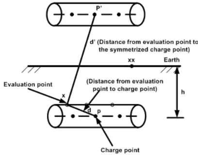
Figure 1 explains the grounding system with grounded electrical equipment and shows the very important parameters in grounding system design.
II. CHARGE SIMULATIONMETHOD FOR ONE-LAYER
SOIL
In the charge simulation method, the actual electric filed is simulated with a field formed by a number of discrete charges which are placed outside the region where the field solution is desired.
Fig. 1. Illustration of the grounding system
Values of the discrete charges are determined by satisfying the boundary conditions at a selected number of contour points. Once the values and positions of simulation charges are known, the potential and field distribution anywhere in the region can be computed easily [7].
The basic principle of the charge simulation method is very simple. If several discrete charges of any type (point, line, or ring, for instance) are present in a region, the electrostatic
potential at any point C can be found by summation of the
potentials resulting from the individual charges as long as the
point C does not reside on any one of the charges. Let Qj be a
number of n individual charges and Φi be the potential at any
point C within the space. According to superposition principle
n
j j ij
i
P
Q
1
(1)where Pij are the potential coefficients which can be evaluated
analytically for many types of charges by solving Laplace or
Poisson’s equations, Φi is the potential at contour (evaluation)
points, Qj is the charge at the point charges.
Because of the ground surface is flat, the method of images can be used with the charge simulation method and the
potential will be characterized for being constant on the grounding grids and its symmetry [8]. The potential coefficients will be as in the following equation;
d
d
P
ij ij ij
'
1
1
4
1
(2)where, dij is the distance between contour point i and charge
point j and d’ij is the distance between the contour point i and
image charge point j’ as shown in Figure 2.
As in Figure 2, the fictitious charges are taken into account in the simulation as point charges. The position of each point
charges and each contour point are determined in X, Y and Z
coordinates where the distance between the contour (evaluation) points are calculated as the following ;
2
2
2i j i j i j
ij
X
X
Y
Y
Z
Z
d
where, Xj, Yj and Zj are the dimensions of the point charge and
Xi, Yi and Zi are the dimensions of the contour point.
After solving equation 1 to determine the magnitude of simulation charges, a number of checked points located on the electrodes where potentials are known, are taken to determine the simulation accuracy. As soon as an adequate charge system has been developed, the potential and field at any points outside the electrodes can be calculated.
Fig. 2. Illustration of the charge simulation technique
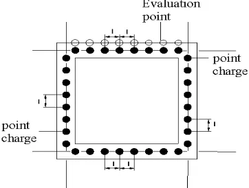
Fig. 3. Distribution of point charges on the grid (1 mesh)
The charge simulation technique is used to get the ground
resistance (Rg), ground potential rise (GPR) and then the
surface potential on the earth due discharging impulse current into ground grid is known. The touch and step voltages are calculated from surface potential. The duality expression is
used to calculate the ground resistance Rg from the next
equation.
1
C
R
V
Q
C
g n
j j
(3)
where, V is the GPR that is defined 1 V, Qj is the charge of
point charge j that used for the calculation, ρ is the soil
resistivity and ε is the soil permittivity.
In this section, some graphs explain the earth surface potential along diagonal profile for the square grid with different number of meshes.
The characteristics of the grid are 50mx50m, the radius of the
grid rods ( r ) is 8 mm, the grid depth (h) is 0.5 m, the
resistivity of the soil () is 100 Ω.m, and the total ground
potential rise (GPR) is defined as 1 V. Figure 4 (a, b) shows the Earth surface potential in 3D and the contour map of this case.
Fig. 4a. ESP/GPR for 64 meshes
Fig. 4b. Contour map for 64 mesh grid
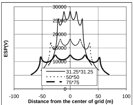
Using CSM for one layer soil, the resistivity of the soil is considered very important parameter in determination of the grounding resistance value, the earth surface potential and then the step and touch voltages. Figure 5 shows that the decrease of the soil resistivity, the decrease of the earth surface potential is observed. Also the side length of grid is very effective parameter in decreasing the grounding resistance and earth surface potential by design a grid with long side, this fact is appear in Figure 6.
0 2000 4000 6000 8000 10000 12000 14000 16000 18000 20000
-100 -50 0 50 100
Distance from the center of grid (m)
E
S
P
(V
)
resistivity=100 ohm.m resistivity=2000 ohm.m
0 5000 10000 15000 20000 25000 30000
-100 -50 0 50 100
Distance from the center of grid (m)
E S P (V ) 31.25*31.25 50*50 75*75
Fig. 6. Effect of the side length in the distribution of earth surface potential along the grid
III. CURRENT SIMULATION METHOD IN TWO-LAYER
SOIL
The representation of a ground electrode based on equivalent two-layer soil is generally sufficient for designing a safe grounding system. However, a more accurate representation of the actual soil conditions can be obtained by using two-layer soil model [9].
As in the Current Simulation Method, the actual electric filed is simulated with a field formed by a number of discrete current sources which are placed outside the region where the field solution is desired. Values of the discrete current sources are determined by satisfying the boundary conditions at a selected number of contour points. Once the values and positions of simulation current sources are known, the potential and field distribution anywhere in the region can be computed easily [7].
The field computation for the two-layer soil system is somewhat complicated due to the fact that the dipoles are realigned in different soils under the influence of the applied voltage. Such realignment of dipoles produces a net surface current on the dielectric interface. Thus in addition to the electrodes, each dielectric interface needs to be simulated by fictitious current sources. Here, it is important to note that the interface boundary does not correspond to an equipotential surface. Moreover, it must be possible to calculate the electric field on both sides of the interface boundary.
In the simple example shown in Figure 7, there are N1
numbers of current sources and contour points to simulate the
electrode, of which NA are on the side of soil A and (N1- NA)
are on the side of soil B. These N1current sources are valid for
field calculation in both soils. At the different soil interface there are N2 contour points (N1 +1,….., N 1+N2), with N2
current sources (N1+1,…..,N 1+N2) in soil A valid for soil B
and N2 current sources (N1+N2 +1,…..,N1 +2N2) in soil B
valid for soil A. Altogether there are (N1+N2) number of
contour points and (N1 + 2N2) number of current sources.
As in Figure 6, h is the grid depth and z is the depth of top
layer soil. In order to determine the fictitious current sources, a system of equations is formulated by imposing the following boundary conditions.
At each contour point on the electrode surface the potential
must be equal to the known electrode potential. This condition is also known as Dirichlet’s condition on the electrode surface.
At each contour point on the dielectric interface, the
potential and the normal component of flux density must be same when computed from either side of the boundary.
Fig.7. Fictitious current source with contour points for field calculation by current simulation method in two-layer soil.
Thus the application of the first boundary condition to contour
points 1 to N1 yields the following equations.
1 1 2,
1 ,
2
1 1, 1 ,
,
1
...
,
1
...
2 1 ! 1 2 1 2 ! 1N
N
i
V
I
P
I
P
N
i
V
I
P
I
P
A N N Nj ij j
N
j aij j
A N
N
N N
j ij j
N
j aij j
(4) where,
' 2 , 2 ' 1 , 1 ' ,1
1
4
1
1
4
,
1
1
4
d
d
P
d
d
P
d
d
P
j i j i a j i a
Again the application of the second boundary condition for
potential and normal current density to contour points = N1+1
to N1+N2 on the dielectric interface results into the following
equations. From potential continuity condition:
2 1 1 2 1 , 1 1 ,
2
0
....
1
,
2 1 2 ! 2 1 1
N
N
N
i
I
P
I
P
N N N N j j j i N N N j j ji
(5)
2
1 1 21
i
J
i
0
for
i
N
1
,
N
N
J
n
n
(6)Eqn. (6) can be expanded as follows:
2 1 1 2 1 , 1 1 1 , 2 2 1 , 2 1
,
1
...
0
1
1
1
1
2 1 2 ! 2 1 ! 1N
N
N
i
I
F
I
F
I
F
N N N N j j j i N N N j j j i N j j j i a
(7) where,
3 ' ' 3 2 2 , 2 3 ' ' 3 1 1 , 1 3 ' ' 3 ,4
4
4
d
zz
zz
d
zz
zz
z
P
F
d
zz
zz
d
zz
zz
z
P
F
d
zz
zz
d
zz
zz
z
P
F
j i j i ij j i j i j i ij j i j i j i a ij a j i a
where, F┴,ij is the field coefficient in the normal direction to
the soil boundary at the respective contour point, ρa, ρ1 & ρ2
are the apparent resistivity and resistivities of soil 1 and 2
respectively and zzi & zzj are the dimension of the contour
point and current source in z direction respectively. Equations 1 to 4 are solved to determine the unknown fictitious current sources.
After solving 4 to 7 to determine the unknown fictitious current source points, the potential on the earth surface can be
calculated by using Eq. 4. Also, the ground resistance (Rg) can
be calculated using the following equation:
1 1 N j gI
V
R
(8)where, V is the voltage applied on the grid which is assumed 1V.
The problem for the proposed method is how the apparent resistivity can be calculated. As in [10], the apparent resistivity for two soil model calculates by the following formula; 1 2 2 1 2 1 1
for
1
1
1
0
h d K ae
(9) 1 2 2 1 1 2 2for
1
1
1
0
h d K ae
(10)where, d0 is the depth to the boundary of the zones, K is the
reflection factor (K=( ρ2- ρ1)/ ( ρ1+ ρ2)) and h is the top layer
depth.
Equations 9 and 10 are valid for the boundary depth greater than or equal the grid depth. But in [11], Eq. 10 is modified
because at very large depth of upper soil layer, resistivity a
given by Eq. 10 tends to 2. This is physically incorrect if the
electrode lies in the upper soil layer, as assumed in [10]. Therefore, Eq. 10 is modified [19] as follows:
1 2 2 1 1 2 1
for
1
1
1
0
h d Ka
e
(11)For finite h and very large d0, resistivity a given by Eq. 11
tends to 1, which is in compliance with physical reasoning.
When the boundary depth is lower than the grid depth, the
apparent resistivity tends to 2. Therefore, by using Eq. 9 and
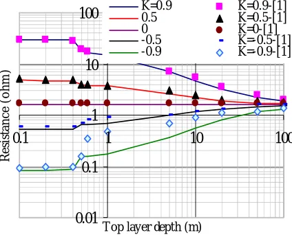
11 for calculating the grounding resistance by Current Simulation Method, the large different between the proposed method results and the results in [12] is observed for K<-0.5 and this shown in Figure 8.
If Eq. 11 is modified as in 12 the results by the proposed method are good agreement with the results in [12].
1 2 15 1 1 2 1
for
1
1
1
0
h d K ae
(12)Figure 9 explains the effect of variation of layer resistivities on the earth surface potential. It is seen that when the lower layer resistivity is decreased, the earth surface potential will decrease and then the step and step voltages. The vertical rods that is connected to the grid play an important roles in decreasing the grounding resistance due to it penetrate the soil to reach to the lower soil with lower resistivity. The effect of vertical rod length is investigated in Figures 10 and 11. A longer vertical rod, a reduction on ESP is observed. The effect of the top layer depth on ESP is illustrated in Figure 12, when the top layer resistivity is greater that that on lower layer, an increase in the top layer depth will result in an increase of the ESP and hence the step and touch voltage. The case study of
Figure 12 is 50m*50m grid with 16 meshes, 1/2=2000/100
0.01 0.1 1 10 100
0.1 1 10 100
T op layer depth (m)
R
e
si
st
a
n
c
e
(
o
h
m
)
K=0.9 K=0.9-[1] 0.5 K=0.5-[1] 0 K=0-[1] -0.5 K=-0.5-[1] -0.9 K=-0.9-[1]
Fig. 8. Relation between 4 meshes grid resistance and the top layer depth
0 1000 2000 3000 4000 5000 6000 7000
-60 -40 -20 0 20 40 60
Distance from center of grid (m)
E
S
P
(V
)
2000/100 ohm.m 2000/20 ohm.m 100/2000 ohm.m
Fig. 9. The effect of variation of layer resistivities on the earth surface potential
0 1000 2000 3000 4000 5000 6000
-100 -50 0 50 100
Distance from center of grid (m )
E
S
P
(V
)
Ver rod length = 6m
Ver rod length=3m
Fig. 10. The effect of vertical rod length on the earth surface potential
0 1000 2000 3000 4000 5000 6000
-60 -40 -20 0 20 40
E
S
P
(V
)
with ver rod 6m
without ver rod
Fig. 11. The effect of presence of vertical rod on the earth surface potential
0 1000 2000 3000 4000 5000 6000 7000
-60 -40 -20 0 20 40 60
E
S
P
(V
)
Distance from center of grid (m) Top layer depth=2m
Top layer depth=3m
Fig. 12. The effect of top layer depth on the earth surface potential
II.
III. IV.BOUNDARYELEMENTMETHOD
In this paper a computer aided design (CAD) system for grounding grids of electrical substations called TOTBEM [6] is presented to get the grounding resistance and earth surface potential. The effect of the vertical rods location on the earth
surface potential and then on Vt and Vs using this technique is
presented in this section.
The characteristics of the grid are 75m*75m, the
number of meshes is 16, the radius of the grid rods (r) is
0.005m, the grid depth (h) is 0.5 m, the resistivity of the soil
is 2000 ohm.m, and the total ground potential rise (GPR) is
0 2000 4000 6000 8000 10000 12000 14000 16000
-150 -100 -50 0 50 100 150
Distance from the center of grid (m )
E
S
P
(
V
)
Fig. 13: The ESP for 16 meshes grid using BEM
V. COMPARISON BETWEEN THE BEM AND CSM
The following case of study is taken to compare between the results by BEM and CSM, the input data about the grid configuration:
Number of meshes (N) = 16, side length of the grid in X direction (X) = 75,50, 31.25m, side length of the grid in Y direction (Y) = 75,50, 31.25m, grid conductor radius = 5 mm, vertical rod length (Z) = 0 (no vertical rod), depth of the grid
(h) = 0.5 m, resistivity of the soil (ρ) = 2000 and 100 Ω.m and
the permittivity of the soil is 9.
The following table I explains that the result from the proposed method is close to the other formula in [1] and also the values of resistance that calculated by BEM[6].
TABLE I
GROUNDING RESISTANCE BETWEEN THE BEM AND CSM AND THE OTHER FORMULAS THAT USED IN IEEE STANDARDS [1]
Rg ohm
Resistivity 2000 ohm.m 100 .m 75m*75m 50m*50m 31.25m*31.25m 50m*50m CSM 12.5 18.45 28.92 0.92 BEM [6] 13.9 20.23 31.36 1.015 Dwight [1] 11.81 17.7 28.35 0.88 Laurent [1] 14.48 21.7 34.7 1.08 Sverak [1] 14.4 21.5 34.06 1.07 Schwarz [1] 12.7 18.54 28.7 0.927
Figure 14 (a, b) explains that the comparison between CSM and BEM for earth surface potential calculation. The Figure explains that the two methods are close to each other for calculating the ESP although the two methods have different techniques.
0 200 400 600 800 1000 1200
-100 -50 0 50 100
E
S
P
(V
)
Distance from the center of grid (m)
CSM BEM
Fig. 14a: Comparison between proposed method and Boundary Element Method for 16 meshes (50m*50m) grid
without vertical rods (=100 .m)
0 5000 10000 15000 20000 25000
-100 -50 0 50 100
E
S
P
(V
)
Distance from the center of grid(m)
CSM BEM
Fig. 14b: Comparison between proposed method and Boundary Element Method for 16 meshes (50m*50m) grid
without vertical rods (=2000 .m)
IV. CONCLUSIONS
The vertical rods play an important role for reducing the grid resistance, the step and touch voltages. The proposed methods (BEM and CSM) that used to calculate the earth surface potential and grounding resistance due to discharging current into grounding grid are efficient. The validation of these methods is satisfying by a comparison between the results from it and the results from the formula in IEEE standard. The proposed methods give a good agreement with the IEEE standard. The two methods give the closest results to each other althought the different techniques are applied in each method.
V. ACKNOWLEDGEMENT
The authors gratefully acknowledge the Taif
University for its Support to carryout this work. It funded this project with a fund number 1732-433-1.
VI. REFERENCES
[3] J. M. Nahman, V. B. Djordjevic, “Nonuniformity correction factors for maximum mesh and step voltages of ground grids and combined ground electrodes,” IEEE Trans. Power Delivery, vol. 10, no. 3, Jul. 1995, pp. 1263-1269.
[4] J. M. Nahman, V. B. Djordjevic, “Maximum step voltages of combined grid-multiple rods ground electrodes,” IEEE Trans. Power Delivery, vol. 13, no. 3, Jul. 1998, pp. 757-761.
[5] S. Serri Dessouki, S. Ghoneim, S. Awad," Ground Resistance, Step and Touch Voltages For A Driven Vertical Rod Into Two Layer Model Soil", International Conference Power System Technology, POWERCON2010, Hangzhou, China, October 2010.
[6] I. Colominas, F. Navarrina, and M. Casteleiro, “Improvement of the computer methods for grounding analysis in layered soils by using high-efficient convergence acceleration techniques” Advances in Engineering Software 44 (2012), pp. 80–91.
[7] N. H. Malik, “A review of charge simulation method and its application,” IEEE Transaction on Electrical Insulation, vol. 24, No. 1, February 1989, pp 3-20.
[8] E. Bendito, A. Carmona, A. M. Encinas and M. J. Jimenez “The extremal charges method in grounding grid design,” IEEE Transaction on power delivery, vol. 19, No. 1, January 2004, pp 118-123.
[9] Cheng-Nan Chang, Chien-Hsing Lee, “ Compuation of ground resistances and assessment of ground grid safety at 161/23.9 kV indoor/tzpe substation”, IEEE Transactions on Power Delivery, Vol. 21, No. 3, July 2006, pp. 1250-1260.
[10] J. A. Sullivan, “Alternativ earthing calculatons for grids and rods,” IEE Proceedings Transmission and Distributions, Vol. 145, No. 3, May 1998, pp. 271-280.
[11] J. Nahman, I. Paunovic, “Resistance to earth of earthing grids buried in multi-layer soil,” Electrical Engineering (2006), Spring Verlag 2005, January 2005, pp. 281-287.