DEVELOPING AND DEPLOYING DATA MINING
TECHNIQUES IN HEALTHCARE
By
SAEED PIRI
Bachelor of Science in Industrial and System Engineering
Amirkabir University of Technology
Tehran, Iran
2008
Master of Science in Industrial Engineering
Sharif University of Technology
Tehran, Iran
2011
Submitted to the Faculty of the
Graduate College of the
Oklahoma State University
in partial fulfillment of
the requirements for
the Degree of
DOCTOR OF PHILOSOPHY
July, 2017
ii
DEVELOPING AND DEPLOYING DATA MINING
TECHNIQUES IN HEALTHCARE
Dissertation Approved: Dr. Tieming Liu Dissertation Adviser Dr. Sunderesh Heragu Dr. Farzad Yousefian Dr. William Paiva Dr. Dursun Delen
iii
Acknowledgements reflect the views of the author and are not endorsed by committee members or Oklahoma State University.
ACKNOWLEDGEMENTS
It has been a long journey since January 2013 when I joined the IEM program at OSU.
From the very beginning, I was surrounded with scholars who guided, inspired, and
helped me reach this point.
First, I would like to thank Dr. Tieming Liu, my advisor for all his help and support in the
past four years, I appreciate everything he did throughout my PhD program. Additionally,
I am grateful for the advice, support, and guidance of my co-advisor Dr. Dursun Delen
who was tremendously helpful and supportive during this process. Completing and
earning my dissertation would not have been possible without his guidance and
dedication.
I acknowledge and appreciate the financial support of CHSI and guidance of its executive
director Dr. Willima Paiva for the past three years. He has been a pleasure to work with
throughout these years. I am also grateful for the advice and support I received from my
committee members, Dr. Sunderesh Heragu, Dr. Farzad Yousefian, and Dr. Arash
Pourhabib. They were all very supportive during the process and were very helpful in
getting me to the finish line.
I would also like to thank my parents. They have always been my greatest inspirations in
all stages of my life and words cannot express how much gratitude I have for all that they
have done for me to ensure I was able to get to the point I am now. I also have to thank
all my family members and friends for their kind support.
Last but not least, I would like to thank the love of my life, Yasamin. Without her
support, it would not have been possible for me to get thorough my PhD. I know I can do
anything with her by my side.
iv
Name: SAEED PIRI
Date of Degree: JULY, 2017
Title of Study: DEVELOPING AND DEPLOYING DATA MINING TECHNIQUES IN
HEALTHCARE
Major Field: INDUSTRIAL ENGINEERING AND MANAGEMENT
Abstract: Improving healthcare is a top priority for all nations. US healthcare expenditure
was $3 trillion in 2014. In the same year, the share of GDP assigned to healthcare
expenditure was 17.5%. These statistics shows the importance of making improvement in
healthcare delivery system. In this research, we developed several data mining methods
and algorithms to address healthcare problems. These methods can also be applied to the
problems in other domains.
The first part of this dissertation is about rare item problem in association analysis. This
problem deals with the discovering rare rules, which include rare items. In this study, we
introduced a novel assessment metric, called adjusted_support to address this problem.
By applying this metric, we can retrieve rare rules without over-generating association
rules. We applied this method to perform association analysis on complications of
diabetes.
The second part of this dissertation is developing a clinical decision support system for
predicting retinopathy. Retinopathy is the leading cause of vision loss among American
adults. In this research, we analyzed data from more than 1.4 million diabetic patients and
developed four sets of predictive models: basic, comorbid, over-sampled, and ensemble
models. The results show that incorporating comorbidity data and oversampling
improved the accuracy of prediction. In addition, we developed a novel “confidence
margin” ensemble approach that outperformed the existing ensemble models. In
ensemble models, we also addressed the issue of tie in voting-based ensemble models by
comparing the confidence margins of the base predictors.
The third part of this dissertation addresses the problem of imbalanced data learning,
which is a major challenge in machine learning. While a standard machine learning
technique could have a good performance on balanced datasets, when applied to
imbalanced datasets its performance deteriorates dramatically. This poor performance is
rather troublesome especially in detecting the minority class that usually is the class of
interest. In this study, we proposed a synthetic informative minority over-sampling
(SIMO) algorithm embedded into support vector machine. We applied SIMO to 15
publicly available benchmark datasets and assessed its performance in comparison with
seven existing approaches. The results showed that SIMO outperformed all existing
approaches.
v
TABLE OF CONTENTS
Chapter
Page
I. INTRODUCTION ...1
Introduction and Motivation ...1
Problem Statements ...5
Research Objectives ...8
Contributions...8
Organization of the Dissertation ...10
II. LITERATURE REVIEW ...11
Rare Rules Association Analysis: The Case of Diabetes Complications ...11
CDSS for Diabetic Retinopathy ...14
Imbalanced Data Learning Algorithms ...17
III. DEVELOPMENT OF A NEW METRIC TO IDENTIFY RARE PATTERNS IN
ASSOCIATION ANALYSIS: THE CASE OF ANALYZING DIABETES
COMPLICATIONS ...22
Methodology ...23
Results ...30
Discussion and Conclusion ...42
IV. A DATA ANALYTICS APPROACH TO BUILDING A CLINICAL DECISION
SUPPORT SYSTEM FOR DIABETIC RETINOPATHY: DEVELOPING AND
DEPLOYING A MODEL ENSEMBLE ...46
Methodology ...46
Results ...61
Discussion and Conclusion ...73
V. DEVELOPING A SYNTHETIC INFORMATIVE MINORITY OVER-SAMPLING
(SIMO) ALGORITHM EMBEDDED INTO SUPPORT VECTOR MACHINE TO
LEARN FROM IMBALANCED DATASETS ...77
Support Vector Machine ...78
SIMO and W-SIMO Algorithms ...82
Numerical Experiments ...87
vi
Chapter
Page
VI. CONCLUSION...105
REFERENCES ...109
vii
LIST OF TABLES
Table
Page
3.1-Hypothetical Dataset H ...25
3.2- Generated rules from Dataset H ...25
3.3-Diabetes complications count and percentage in the data ...29
3.4-Comorbidity index value by race/ethnicity ...31
3.5- Comorbidity index value in rural vs urban diabetic patients ...32
3.6- Comorbidity index value by gender ...32
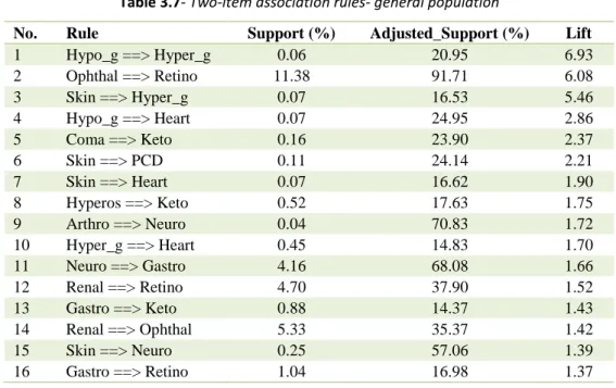
3.7- Two-item association rules- general population ...37
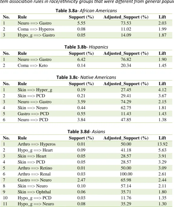
3.8- Two-item association rules in various demographic groups ...39
3.9-Three-item association rules- general population ...42
4.1- Demographic variables ...62
4.2- Lab procedure variables ...62
4.3- Comorbidity variables ...63
4.4- Set 1 - Basic models’ results...65
4.5- Set 2 - Comorbid models’ results ...66
4.6- Set 3 - Over-sampled models’ results ...67
4.7- Set 4 - Ensemble models’ results ...71
5.1-Notations for SIMO and W-SIMO algorithms ...86
5.2 -Benchmark datasets characteristics ...91
5.3- Performance of imbalanced data learning approaches (using G mean) ...93
5.4- Performance of imbalanced data learning approaches (using AUC) ...94
5.5-Average difference between our algorithm and other approaches ...96
5.6-Overall ranking on linear SVM ...96
5.7-Overall ranking- SVM-RBF kernel ...96
5.8-Overall ranking on logistic regression ...96
5.9- Overall ranking on decision tree ...96
5.10-The performance of best approach in each machine learning technique ...97
5.11- Imbalanced gap and average # of synthetically generated data points ...98
5.12- Sensitivity analysis on SIMO parameters ...100
viii
LIST OF FIGURES
Figure
Page
1.1- Three analytics levels-descriptive, predictive, and prescriptive ...3
3.1- Final dataset structure ...30
3.2-Comorbidity index value by race/ethnicity ...31
3.3a- Comorbidity index value in rural vs urban diabetic patients ...32
3.3b- Comorbidity index value by gender ...32
3.4- Diabetes complications' prevalence by race/ethnicity ...33
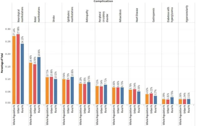
3.5-Diabetes complications' prevalence: rural versus urban ...35
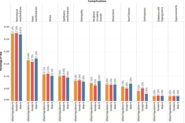
3.6-Diabetes complications' prevalence: females versus males ...36
4.1- A simplified conceptual data model for Cerner Health Facts ...48
4.2- Data preparation steps ...49
4.3- Modeling procedure ...52
4.4- Two-layer perceptron neural network ...53
4.5- Predictive model sets ...56
4.6- Synthetic minority over-sampling technique (SMOTE) ...57
4.7- AUC comparison among modeling techniques and modeling sets ...68
4.8 - ROC charts of modeling techniques in different sets ...69
4.9- Variable importance ranking in detecting diabetic retinopathy ...72
5.1- Linear SVM hyperplane ...79
5.2- SIMO algorithm mechanism (simplified)...84
5.3- Confusion matrix ...88
5.4- ROC chart ...90
1
CHAPTER I
INTRODUCTION
1.1.Introduction and Motivation
Improving healthcare is a top priority for all nations. In 2014, US healthcare expenditure was $3 trillion, or $9,523 per person. In the same year, the share of GDP assigned to healthcare
expenditure was 17.5% [1]. These statistics shows the importance of improving the healthcare delivery system.
Diabetes is one of the most serious and prevalent chronic conditions affecting approximately 415 million people worldwide, with this number is expected to grow to 642 million by 2040 [2]. The situation is particularly dire in the U.S., which has the highest prevalence of diabetes of all developed nations. Approximately 86 million adults aged 20 years and older (37%) were
diagnosed as pre-diabetic between 2009 and 2012. By 2014, the estimated number of adults with diagnosed or undiagnosed diabetes topped 29 million, representing about 9% of the U.S. adult population (National Diabetes Statistics Report, 2014). Minority racial/ethnic groups have higher rates of diabetes than non-Hispanic whites, with Native Americans having the highest rate at nearly 16%, followed by African American (13.2%), Hispanics (12.8%), Asian Americans (9%)
2
and Caucasians (7.6%). Each year, approximately 1.4 million people are diagnosed with either type 1 or type 2 diabetes, making it the nation’s seventh leading cause of death in 2010. The cost of diabetes in America in 2012 was approximately $245 billion, which included about $69 billion in indirect costs related to impairment, job loss, and premature death.
In recent years, due to modern healthcare technology, a large amount of data from various sources, such as patient care, as well as compliance and regulatory requirements has become available [4]. The digitization of this data has been happening rapidly in the recent years [5]. The extensive availability of healthcare data, as well as advances in the area of data mining and machine learning, has generated the interesting field of healthcare analytics. The development of decision support systems by data analysts with the aid of clinical experts’ knowledge has eased the burden on physicians and clinicians and smoothed clinical procedures. Analyzing healthcare data and applying machine learning techniques in this area have several benefits: patients can be stratified based on the severity of a particular disease or condition and, consequently, suitable treatments can be provided for each group; risk factors of different diseases can be identified, leading potentially to better health management; and diseases can be detected at early stages, allowing for appropriate interventions and treatments. For a comprehensive discussion about healthcare analytics, its promises and its potentials we refer readers to [5].
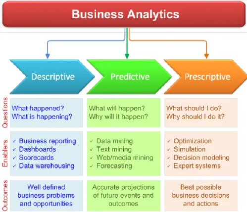
Similar to other domains, three types of analytics can be conducted in healthcare: descriptive, predictive, and prescriptive. Most of the analytics projects start with descriptive analytics [6]. Descriptive analytics tells us what has happened in the past and what is going on at the present. In descriptive analytics, hypotheses are tested, and trends are identified. Descriptive analytics could lead to discovering interesting patterns in the data. The next step in analytics is predictive analytics. Predictive analytics tells us what is going to happen in the future. In predictive analytics, by using statistical and machine learning models to analyze historical data, the relationship between the target and predictors can be detected [7]. The final step in an analytics
3
project is prescriptive analytics. In this step, analysts use optimization techniques to identify the best course of action. In Figure 1.1, different levels of analytics can be seen [8].
Figure 1.1- Three analytics levels-descriptive, predictive, and prescriptive. Adopted from Real-World Data Mining: Applied Business Analytics and Decision Making, by D. Delen, 2015: FT Press (a Pearson Publishing
Company). Adapted with permission
Discovering the affinities and associations among various items has long been of interest to managers and data analysts. Association rule mining (or market basket analysis in the marketing and business literature) is a data mining method that aims to reveal the association/affinity patterns/rules among various items (objects or events) that occur together. We can enumerate several implications for association rule mining. In the retail industry, it facilitates finding solutions for assortment planning, coupon design, and product discounting [9]. In health care settings, association rule mining may help answer questions such as whether the presence of a particular health condition increases the probability of developing other conditions and which
4
preventive measures could best reduce risk of complications. These questions can be addressed through an understanding of the associations among different complications.
One critical challenge in healthcare domain is detecting the disease in early stages. One of the major complications of diabetes that has not received enough attention is diabetic retinopathy. This complication is the most common cause of vision loss among people with diabetes and a leading cause of blindness for American adults. According to the 2014 National Diabetes
Statistics Report, between the years 2005 and 2008, 4.2 million of American diabetics aged 40 or older suffered from diabetic retinopathy. Among patients who have had diabetes for up to 20 years, almost all type І and more than 60% of type ІІ diabetics develop retinopathy [10]. This complication is caused by damage to the blood vessels of retina, the light-sensitive tissue at the back of the eye. At its early stages, diabetic retinopathy may be asymptomatic or only show mild vision problems, but if it is not diagnosed and treated in time, it can eventually cause blindness.
Another challenge that data analysts face in the healthcare domain as in many other domains is dealing with imbalanced datasets. A dataset is called imbalanced when the distribution of different classes in the data is not similar. For instance, in the case of two-class data, there are many more examples of one class (negative examples) compared to the other class (positive examples). Let us call the class with fewer examples the minority class, and the class with more examples the majority class. The imbalanced datasets are very common in real-life problems, especially in pattern recognition problems. For example, if a sample of people were tested for a specific disease, only a small portion of them would actually have the disease. Another example is credit card fraud detection where only a few numbers of transactions in the whole sample of transactions are actually fraud [11].
In imbalanced datasets, the prediction accuracy, especially for the minority class, is a critical challenge. When the standard machine learning techniques are applied to the imbalanced data, the
5
result will be in favor of the majority class, i.e. a big portion of the minority class examples will be classified as the majority. In real world applications, the detection accuracy of the minority class is critically important because the minority class usually is the class of interest. Thus, misclassifying the minority class has much higher cost compared to misclassifying a majority class example. To make it clearer, compare the cost of misclassifying a cancerous patient as non-cancerous to the cost of misclassifying a non-non-cancerous as non-cancerous; in the former case, the misclassification may lead to death of a person but in the latter case, there will be some more tests and screenings.
1.2.Problem Statements
One of the most critical problems in association rule mining is the rare item problem. This
problem emerges when there are items that occur rarely compared to items that are more frequent. For instance, in retail, purchases of items such as electronics or jewelry are likely rarer than grocery purchases. Rare items, however, may be equally as important as frequent items or even more so. In health care, some complications may not be as frequent as other complications, but they may be more critical or even fatal. Therefore, it is important to recognize and discover the association patterns among rare items as well as the association patterns between rare and frequent items. Any association rule that includes a rare item is called a rare rule. Discovering rare rules is a critical challenge in association analysis. In classical association rule mining, a minimum support is specified to extract the association rules. Support of a rule specifies the fraction of a population for which the rule is true. Setting a high threshold for support may lead to losing rare association rules. On the other hand, specifying a low threshold for support will lead to over generating association rules. Therefore, the problem statement is “how to retrieve and discover rare association rules without over-generating association rules?”
6
Diabetes typically leads to several complications, often presenting simultaneously. The American Diabetes Association (ADA) classifies these conditions as: skin complications, eye complications (retinopathy), neurological manifestations (neuropathy), foot complications, diabetic ketoacidosis (DKA) and ketones, renal manifestations (nephropathy), high blood pressure (hypertension), stroke, hyperosmolar hyperglycemic nonketotic syndrome (HHNS), gastroparesis, heart disease, stroke, and mental health. The existence of more than one distinct condition in a patient is defined as comorbidity [12]. Comorbidity is highly prevalent in diabetics. Research shows that between 1999 and 2004, only 14% of type 2 diabetic patients were not diagnosed with any additional comorbid conditions [13]. The benefit of considering comorbidities as opposed to studying different diseases in isolation has been showed by many researchers ([14], [15], [16], [17], and [18]). The high prevalence of comorbid conditions among diabetics and the benefits of studying comorbidities shown by other researchers motivated us to study the comorbidity in diabetes and conduct association analysis among its complications. The problem statement here is “is there any strong and interesting association among complications of diabetes?”
Although retinopathy is preventable and existing treatments can slow down the disease progress, vision loss that happens in the late stages of retinopathy cannot be restored. Thus, it is critical to diagnose this complication as early as possible. The current method for diagnosing diabetic retinopathy is a comprehensive eye examination in which after a patient’s eye is dilated, an ophthalmologist examines the retina with an indirect ophthalmoscope and a special lens. Unfortunately, and despite the high prevalence of retinopathy, the annual diabetic retinopathy evaluation has one of the lowest rates of patient compliance for several reasons. First, many patients do not seek proper medical attention because this disease is asymptomatic at the early stages; second, availability of ophthalmologists is low or even nonexistent in many areas, especially in rural communities; and third, many patients find the necessary eye dilation
7
are undiagnosed (National Eye Institute report, 2015). Therefore, the rising prevalence of diabetes, coupled with barriers to ophthalmological screenings that lead to a high rate of undiagnosed diabetic retinopathy patients, create an urgent need for a tool to detect this
complication. To be useful, this tool should be non-invasive, readily available to diabetic patients, validated on a large number of cases, and eliminate the need for specialized equipment that is not universally available. This study sets out to employ an analytics approach on data collected during routine primary care visits to fills this gap. Specifically, we build a clinical decision support system (CDSS) for prediction of diabetic retinopathy that satisfies the aforementioned requirements for diagnostic tools. Our problem statement in this research topic is “How to detect diabetic retinopathy at early stages when retina images are not available?”
To develop the CDSS for diabetic retinopathy, we have applied several machine learning techniques such as neural networks, logistic regression, decision tree and random forest.
Ensemble models are learning approaches that combine multiple single classifiers and then make the final classification decision by an averaging or voting mechanism [19]. Use of ensemble models in several studies in the literature, including the studies that used lab and demographic data to predict diabetic retinopathy, points out to the complexity of this problem domain. Ensemble models have the benefit of being more robust than single models [20], and therefore, improve prediction accuracy. For this reason, we also employ an ensemble modeling approach in developing our CDSS. Specifically, we develop a heterogeneous confidence margin ensemble and illustrate how it outperforms the existing ensemble techniques. In this research topic, the problem statement is “how to improve the prediction accuracy of single classifiers through developing an efficient ensemble approach?”
There are various remedies for the imbalanced data learning problem. One of these remedies is to modify the imbalance ratio in the dataset. Decreasing the imbalanced ratio can be achieved through either under-sampling the majority class, i.e. removing some portion of data that belong
8
to the majority class; or over-sampling the minority class, i.e. generating synthetic data points that belong to the minority class. In this research topic, the problem statement is “how to address the problem of learning from imbalanced data, by developing an efficient over-sampling algorithm?”
1.3.Research Objectives
Our research objectives in this dissertation are as follows,
Developing a new assessment metric to discover rare rules in association analysis
Discovering the potential existing associations among complications of diabetes by applying association analysis
Developing a CDSS to detect diabetic retinopathy using lab data collected during a routine diabetic primary care visit
Developing a novel ensemble approach to further improve the prediction accuracy of single classifiers
Developing an over-sampling algorithm embedded into support vector machine to enhance the performance of machine learning techniques when applied to imbalanced datasets
1.4.Contributions
In this research, we have three topics. First topic is “developing a new metric to identify rare patterns in association analysis: the case of analyzing diabetic complications”. Second topic in this dissertation is “a data mining approach to build a clinical decision support system for diabetic retinopathy: developing and deploying a model ensemble”. Finally, the third topic is “developing a synthetic informative minority over-sampling (SIMO) algorithm embedded into support vector machine to learn from imbalanced datasets.”
9
In the first research topic, our contributions to the fields of decision support systems and medical informatics are twofold. At the methodological level, we introduced adjusted_support, a new assessment metric for association rule mining that addresses the rare item problem. By using adjusted_support, we will be able to address the problem of rare items by extracting rare rules without over-generating association rules. At the application level, we performed association rule mining on the complications of diabetes by applying the adjusted_support metric. Our findings in this research shed light on the association patterns among diabetes complications, which has not received enough attention in the literature.
Second research study contributes to the data mining and medical decision support literatures from three perspectives: methodology, data management, and application. In the methodological aspect, we develop and evaluate a novel approach in building ensemble models. This approach aggregates the predictions of individual models by calculating a weighted confidence margin across all models. However, in contrast to the existing weighted averaging ensembles that assign weights to individual models based on their overall prediction performance, our confidence margin ensemble assigns varying weights to the constituting models. These weights are calculated for each observation in the data and are based on the distance between the estimated probabilities of records and the decision cut off point. We show how this approach improves the accuracy of decisions made by our CDSS. From the data management perspective, we processed a very large transactional database of clinical encounters and aggregated the observations at the patient level. This enabled us to create a single data set containing comorbid conditions of patients to develop an accurate picture of their health status. Consequently, our CDSS is able to consider a larger number of risk factors and provides a more realistic depiction of the coexistence of chronic diseases. Finally, in the application aspect, we develop an accessible,
10
among diabetics. This CDSS reduces direct and indirect medical costs of the healthcare system in the US and more importantly, saves eyesight for a large number of citizens.
In the third research topic, we propose a novel over-sampling algorithm integrated with support vector machine (SVM). We can numerate several advantages for our proposed algorithm. First, it is embedded into a powerful classifier, i.e. SVM, and therefore better results are expected
compared to other pre-processing approaches. Second, we conduct over-sampling rather than under-sampling that may lead to information loss due to discarding a fraction of data. Finally, we perform the over-sampling only on the informative minority examples. In this way, we generate the least amount of synthetic data points; therefore, the distribution of the training data will not change dramatically. In addition, because the amount of synthetic generated data is much less compared to other existing methods such as SMOTE, Borderline SMOTE, Safe-Level SMOTE, and Cluster-SMOTE, the computational cost of training machine learning techniques will be lower.
1.5.Organization of the Dissertation
The remainder of this dissertation is organized as follows. The second chapter contains the literature review on the three topics that are covered in this research. The third chapter presents the association analysis method and its implementation on diabetes complication. In Chapter 4, different stages of developing a CDSS for diabetic retinopathy is described and the results of the developed predictive and ensemble models are provided. Chapter 5 presents our developed over-sampling algorithm, SIMO. This algorithm is evaluated compared to other existing approaches and the results are provided in Chapter 5. Finally, in Chapter 6, we summarize and conclude the dissertation.
11
CHAPTER II
LITERATURE REVIEW
In this chapter, we review the related literatures for the research topics in this study. First, we provide the literature review for association analysis and the rare rule problem. We also review the studies related to the application of association analysis on diabetes complications. Then, we discuss the related studies to the diabetic retinopathy CDSSs and ensemble models. Finally, we review the studies in the domain of imbalanced data learning.
2.1. Rare Rules Association Analysis: The Case of Diabetes Complications
In recent years, the application of analytics and data mining in health care has received much attention. Although association analysis has been one of the popular data mining methods applied to health care data, its application to studies of diabetes complications, especially rare
complications, is still limited. Agrawal, et al. [9] introduced association analysis for the first time. They studied associations among items in a large customer transaction dataset. Following their work, association analysis has been applied to many domains, such as bioinformatics ([21], [22], [23]), social domain ([24], [25], [26]), and earth science ([27], [28]).
12
One of the components of association analysis is assessing rules such that only the most useful ones are retained. Several assessment measures, termed interestingness metrics, exist for evaluating rules and filtering out the least useful. Two traditional measures, support and confidence, will be described in detail in Chapter 3. Several other interestingness metrics for association rules were introduced by researchers, such as h-confidence by Xiong, et al. [29], NConf by Liu, et al. [30] and relative-confidence by Yan, et al. [31]. Tan, et al. [32] extensively reviewed 21 metrics for association patterns and described their usefulness in different
application areas. Various association analysis techniques and their properties were reviewed by Kotsiantis and Kanellopoulos [33].
Rare item problem is one of the important challenges in association analysis. Theoretically studying the rare item problem in association analysis started by Liu, et al. [34]. They proposed a multiple min-support approach in which every item in the data has its own min item support (MIS). MIS is specified by comparing a lowest allowable support and the support of the item times a parameter, 𝛽. In this way, rare items have lower min-support compared to frequent items, thus they will not be ignored in the rule generation procedure. There are two are main downsides of this approach. First, specifying MIS when the number of items in the dataset is large is a tedious job, and second, determining the optimal value of 𝛽 is not easy. To address these issues, Yun, et al. [35] introduced relative support. Their formula does not include the parameter 𝛽, therefore they did not have the challenge of determining the optimal value for 𝛽. Nevertheless, their approach still requires specifying multiple suitable min-support for various itemsets.
Wang, et al. [36] also introduced a framework to address the rare item problem. Similar to the two previously mentioned studies, they assigned different min-support to various itemsets by tracking the dependency chain of itemsets in generating the itemset. While other multi min-support approaches focus on the frequency of items, the approach developed by Seno and Karypis [37] focuses on the length of the itemset, i.e., the itemsets with more items have lower
min-13
support while itemsets with fewer items have higher min-support. Any-confidence,
all-confidence, and bond were introduced by Omiecinski [38] as alternatives for supports in rare item association analysis. Adjusted_support is similar to any-confidence in 2-item rules. These metrics are effective for rules that all items are rare, but they are not effective for rules containing both rare and frequent items. Kiran and Re [39] proposed an improved multiple min-support approach for extracting the rare association rules. Their approach requires specifying multiple minimum support, which is inconvenient compared to a single minimum adjusted_support in real-world application. For a comprehensive review of existing methods and metrics for rare item association analysis, we refer readers to [40].
Several researchers have applied association analysis to diabetes. Simon, et al. [41], Simon, et al. [42], Ramezankhani, et al. [43], and Kamalesh, et al. [44] applied association analysis to assess the risk of developing diabetes. Shin, et al. [45] analyzed the data of 5,022 patients diagnosed with essential hypertension and Valent, et al. [46] analyzed the data of 9,358 diabetic patients. By applying association analysis, they showed that essential hypertension and diabetes mellitus were strongly associated. This result is not surprising since about 71% of diabetic patients have hypertension [3]; thus, this association pattern cannot be considered very useful or interesting. Kim, et al. [47] analyzed the data of 20,314 diabetic patients in South Korea and assessed the associations among various diseases and type 2 diabetes. They found strong associations between diabetes and hypertension; diabetes, hypertension, and stroke; and diabetes, hypertension, and dyslipidemia. However, the relatively small number of patients as well as the limitation of race to Asians diminishes the reliability and generalizability of their results. Therefore, there is an urgent need for a comprehensive study of the associations among diabetes complications using a large dataset that represents the diversity of diabetic patients. Our study fills this gap in the literature by performing association analysis on complications associated with diabetes and introducing a new interestingness assessment metric that captures both rare and frequent association patterns.
14 2.2. CDSS for Diabetic Retinopathy
Even though CDSSs based on EMR data have been broadly used by practitioners in recent years, its implementation in the field of ophthalmology is still limited [48]. This dearth exists while several researchers have studied the relationship between diabetic retinopathy and different potential risk factors. For instance, Karma, et al. [49] studied the existence of diabetic retinopathy in 328 diabetic patients using ophthalmoscopy and wide field fundus photography and tried to identify the association between diabetes duration and other risk factors, such as nephropathy and coronary disease. In another study, Klein, et al. [50] measured the relationship between
retinopathy and hyperglycemia by studying 1878 diabetics.
Most of the existing CDSSs for diabetic retinopathy use image processing algorithms. While these algorithms facilitate early detection of diabetic retinopathy, they require an image of the retina. Therefore, although they ease the burden of assessing the images of retina, they fail to address the evident barrier of patients’ access to specialists. Examples of studies that belong to this category are (Kahai, et al. [51], Paunksnis, et al. [52], Marsolo, et al. [53], Tsai, et al. [54], Noronha, et al. [55] Bursell, et al. [56], Kumar and Madheswaran [57], and Xiao, et al. [58]). We refer the readers to Mookiah, et al. [59] for a comprehensive review of research in this category. The other category of CDSSs for diabetic retinopathy includes those matched with lenses or an ophthalmoscope that can be used on a smartphone. Prasanna, et al. [60] proposed a portable smartphone-based CDSS that requires attaching an ophthalmoscope to a smartphone to capture fundus images, and captured images will be processed by the algorithm installed on the smartphone. Bourouis, et al. [61] also proposed a smartphone-based algorithm integrated with microscopic lenses used to capture retinal images. Their CDSS uses a neural network model to analyze such images and provide the results. Despite all the benefits of these algorithms,
15
additional equipment is still required for retinal imaging, which, for many diabetics and primary care providers, may be cost-prohibitive or unavailable.
Many research projects have studied the association of retinopathy and different lab tests. For instance, the association of retinopathy and hemoglobin A1c has been shown in several studies ([62], [63], [64]). Researchers have also studied the relationship between cholesterol and retinopathy and have found the two to be related ([65], [66]). The Diabetes Control and
Complications Trial (DCCT) and the U.K. Prospective Diabetes Study (UKPDS) have shown that controlling the glucose level could reduce the risk of retinopathy [67]. Other studies have shown that retinopathy and hypertension are associated [68]. Besides blood tests, some urine tests such as proteinuria are shown to be associated with retinopathy [69].
While these studies show the potential for developing tools that can detect or predict retinopathy using lab results, only a few studies have used lab and demographic data to detect diabetic retinopathy without requiring retinal imaging. Skevofilakas, et al. [70] developed a CDSS using data from 55 type І diabetic patients to predict the risk of diabetic retinopathy. They applied classification-based Rule Induction with C5.0, Hybrid Wavelet Neural Network (HWNN), Classification and Regression Tree (CART), and neural network, and merged their results using a voting mechanism. In another work, Balakrishnan, et al. [71] used data from 140 diabetic patients in Malaysia to build a diabetic retinopathy predictive system, which employed a voting
mechanism to select the final outcome from the results of decision tree and case-based reasoning (CBR).
Although these two research projects did not use any retinal images to predict the risk of diabetic retinopathy, they are limited in a number of ways. First, they are based on small samples (55 in the first and 140 patients in the second study). Second, they consider a limited number of risk factors. These charactreistics not only contribute to lack of a comprehensive image of the
16
patients’ health status, but also make the final results less generalizable. Additionally, while according to the NIH statistics, 95% of the diabetics are type ІІ, the first study has only focused on type I diabetic patients. Research shows between 74.9% to 82.3% of type I diabetics have retinopathy [72]. Therefore, the baseline model for predicting retinopathy among type I diabetics will have an accuracy of about 80%. Moreover, almost all type І diabetic patients who have had the disease for 20 years develop this vision complication.Thus, despite the first study’s high accuracy (98%) in predicting retinopathy among type I diabetic patients, it does not address the more important problem of detecting retinopathy in type II diabetics. This limitation is addressed in the second study, but with an overall accuracy of 85%, it leaves room for improvement. Therefore, another promise of the current effort is to develop a model that addresses the limitations of the extant literature, while improving upon their results.
Ensemble models for supervised learning were first introduced by Tukey [73] and have since been studied by many researchers. At a high level, there are two categories of ensemble models: homogeneous and heterogeneous ensembles. Homogeneous ensembles combine multiple variations of a single classifier technique. Ensembles in this category use such algorithms as Bagging and AdaBoost to manipulate the training dataset and to develop multiple training datasets. These training datasets will be used by a data mining technique such as decision tree, and at the end, a voting or averaging mechanism will be used to make the final prediction using the outputs of single classifiers [19]. One of the most famous ensemble models in this category is random forest. Heterogeneous ensembles, on the other hand, combine various single classifiers (that are built using different data mining techniques) on the same training dataset. Simple average, weighted average, and voting based ensembles belong to this category [74]. A comprehensive review of ensemble techniques can be found in Rokach [75]. In this study, we developed a novel heterogeneous ensemble approach that will be explained in Chapter 4.
17 2.3.Imbalanced Data Learning Algorithms
Studying the imbalanced data classification has received a considerable amount of attention in recent years. He and Garcia [76] classified the different approaches of analyzing imbalanced data into four main classes,
- Sampling methods - Cost-sensitive methods
- Kernel-based methods and active learning methods
- Other methods such as, one-class learning, novelty detection, etc.
Sampling methods: The aim of the sampling methods is to reach some degree of balanced distribution in the dataset. These methods can be categorized into two major streams, those that under-sample the majority class and those that over-sample the minority class. In under-sampling methods, some parts of the majority examples are removed. As a result, the distribution of the classes will be more balanced. The simplest method in this category is the random under-sampling. There is not any specific mechanism for under-sampling in this approach and it functions merely randomly. Other under-sampling approaches such as BalancedCascade and EasyEnsemble presented by Liu, et al. [77] are called informed under-sampling. In
EasyEnsemble, several samples of the majority class data are taken and combined with minority class data. Multiple models are built based on these datasets, and at the end an ensemble model makes the final decision. The main criticism of the under-sampling methods is that by removing some parts of the data, potential important information in the data can be lost.
Over-sampling on the other hand, is to re-sample or generate extra examples of the minority class. The most basic over-sampling method is random over-sampling in which minority examples in the data are randomly duplicated. The main downside of random over-sampling is over-fitting. Another major approach in over-sampling is synthetic data generation. SMOTE
18
(Synthetic Minority Over-Sampling Technique) is one of the most well-known methods in synthetic data generation. In this method, synthetic data points are generated on the line connecting the minority samples to their k nearest minority class neighbors [78]. The major drawback in SMOTE is that it may lead to over-generalization.
There are extensions to the SMOTE that tried to improve the performance of this technique. Han, et al. [79] proposed a synthetic over-sampling method named Borderline-SMOTE. In this
method, only a subset of minority data points is over-sampled by SMOTE technique. Those minority data points are located near the border of two classes.Borderline minority data points are identified as minority examples that most of their nearest neighbors belong to the majority class. On the other hand, Bunkhumpornpat, et al. [80] introduced a method named Safe-Level SMOTE. This method calculates a parameter called safe-level. The greater that a safe-level is for a minority example shows that example is farther away from the borderline. After identifying the minority examples in safe regions, those data points will be over-sampled using SMOTE. Cieslak, et al. [81] introduced the cluster SMOTE method. This method first clusters the minority
examples, and then over-samples data points within each cluster by applying SMOTE.
Barua, et al. [82] proposed a majority weighted minority oversampling technique that first identifies hard to learn minority examples by considering their distance from the majority neighbors, and then it over-samples those examples using a clustering approach. There are other studies in the area of synthetic data generation ([79], [83], and [84]). Generally speaking, synthetic oversampling significantly improves the classification accuracy, especially for the minority class. Another advantage is that by generating the synthetic minority data (not simply replicating existing minority data), the minority region is generalized and overfitting can be avoided [85]. For a more comprehensive review of the sampling methods, we refer readers to He and Garcia [76].
19
Cost-sensitive methods: Unlike sampling methods that alter the distribution of the data through either generating synthetic minority data points or removing some portion of majority data points, the idea of cost-sensitive methods is based on the different misclassification costs for different classes in the dataset. Usually the cost of misclassifying the minority class is much higher than the majority class misclassification [86]. To perform cost-sensitive methods, a matrix, called cost matrix is required. This matrix shows the misclassification cost for different classes in the dataset [87]. The main concern about cost-sensitive methods is that in most of the situations the exact misclassification cost related to various classes is unknown [88].
There are three major categories in cost sensitive approaches [76]. The first category includes techniques that assign various weights to the examples in the dataspace. Methods in this category are motivated by the AdaBoost algorithm [89]. AdaBoost is a meta-algorithm that begins with the original dataset and trains a model on this dataset. Incorrectly classified examples are identified, and in the next iteration more weight (higher error cost) will be assigned to them. In this way, more focus will be on the examples that are misclassified. This process repeats and the classifier performance improves. The second group encompasses approaches are those that use ensemble schemes integrated with cost-sensitive approaches. Many of the research studies in these two categories have combined various weighting and adaptive boosting techniques. For instance Sun, et al. [90] and Fan, et al. [91] proposed algorithms for updating the weights in AdaBoost in imbalanced data learning. Lee, et al. [92] used SVM to adjust the weights of the examples in AdaBoost to learn from imbalanced data. In the third category, cost-sensitive methods incorporate the misclassification costs directly into the classifiers. Cost-sensitive decision tree [93], cost-sensitive neural networks [94], and cost-cost-sensitive SVM [95] are in this category.
Kernel-based methods: Kernel-based methods are mostly integrated with SVM. Many researchers have studied imbalanced data learning through support vector machine. Wu and Chang [96] developed a boundary-alignment algorithm, which makes a change in the kernel function to move
20
the boundary toward the negative instances. Akbani, et al. [97] proposed an algorithm by
integrating the different error cost method [95] and the SMOTE over-sampling method, however they performed the SMOTE over-sampling independent from the SVM model. Wang and Japkowicz [98] applied boosting and asymmetric error cost for minority and majority classes. Mathew, et al. [99] proposed a kernel-based SMOTE for SVM. In their approach, the over-sampling through the SMOTE technique happens in kernel feature space. Yu, et al. [100] developed the SVM-OTHR algorithm. In this algorithm, they adjusted the decision threshold by moving the decision hyperplane toward the majority class data.
Tang and Zhang [101] proposed a granular SVM with repetitive under-sampling. They utilized SVM for under-sampling in a way that they repeatedly developed SVM models and each time discarded the negative (majority class) support vectors from the data. Even though they performed the under-sampling integrated with the SVM, the problem of losing potential
important information by under-sampling still exists. As Akbani, et al. [97] showed in their paper, under-sampling the majority class may decrease the total error, but it usually deteriorates the performance of the SVM on the test data, because it fails to approximate the orientation of the ideal hyperplane. Batuwita and Palade [102] suggested an over-sampling method in which they selected the majority examples near the boundary as the informative negative data points, and then they randomly over-sampled the minority examples to have relatively balanced data. This work can be critiqued in two ways. First, they focused on the informative majority examples, while the primary interest in imbalanced datasets is on the minority examples, therefore the focus on the informative majority examples may lead to even more bias toward the majority class. Second, they simply applied random over-sampling that is not as powerful as synthetic data generation methods and may lead to over-fitting. The two former studies did not compare their model’s performance with other exiting methods; therefore, it is not easy to comment on generalizability and efficiency of their model. [103] proposed a preprocessing approach using
21
SVM for imbalanced data. In their approach, they first trained SVM on the original data, and then replaced the actual target variable value by the SVM predicted value. They claimed that SVM will classify a portion of the majority examples as minority, and therefore the processed data will have a more balanced distribution. Their claim is questionable, because in imbalanced data learning most of the time there is poor accuracy on minority class and good accuracy on majority. This means that most of the minority examples are misclassified as majority not the other way around. They tested their approach only on one dataset; therefore, their results could be because of the characteristics of that special dataset.
22
CHAPTER III
DEVELOPMENT OF A NEW METRIC TO IDENTIFY RARE PATTERNS IN ASSOCIATION ANALYSIS: THE CASE OF ANALYZING DIABETES COMPLICATIONS
In this chapter, we present the methodology of association analysis and our developed metric, adjusted_support. Following that we provide the results of applying adjusted_support and association analysis to complications of diabetes. The number of co-existing complications among diabetic patients could be a meaningful index to evaluate their health status. In this study, we defined comorbidity index as the mean number of co-exiting complications in a diabetic patient. Besides association analysis, we also performed a comorbidity analysis on diabetic patients by calculating their comorbidity index and compared the comorbidity index of patients in different demographic groups. This analysis will provide insight on the comorbidity status of diabetics at a more granular level and can lead to better decision making by healthcare administrative professionals and clinicians. In addition, we studied the prevalence of diabetes complications among various demographic groups.
23 3.1. Methodology
In this section, we start with briefly describing association analysis, define its common parameters and metrics, and explain the algorithmic extent of our proposed rare item/patterns identification metric.
Let 𝐼 = {𝑖1, 𝑖2, … , 𝑖𝑛} be the set of all items (in our study, items are various diabetes
complications), and 𝑅 = {𝑟1, 𝑟2, … , 𝑟𝑁} be the set of all records in our data (each record
corresponds to each patient and contains the patient’s complications). Let 𝑋 be a subset of 𝐼, i.e., a subset of items (diabetes complications), then 𝑋 is called an itemset (𝑋 = {𝑖1, 𝑖2, … , 𝑖𝑘). An
itemset with 𝑘 items is called k-itemset. Every record, 𝑟𝑖, includes a subset of items
(complications) in 𝐼, thus each 𝑟𝑖 is an itemset (𝑟𝑖 ⊆ 𝐼). Suppose itemset 𝑋 contains the following
complications: retinopathy, nephropathy, and neuropathy. The support count for 𝑋 is the number of records that include items in 𝑋. The support count for 𝑋 is denoted by 𝑠𝑢𝑝𝑝𝑜𝑟𝑡_𝑐𝑜𝑢𝑛𝑡(𝑋), and is calculated as in Equation 3.1.
𝑠𝑢𝑝𝑝𝑜𝑟𝑡_𝑐𝑜𝑢𝑛𝑡(𝑋) = |{𝑟𝑖|𝑋 ⊆ 𝑟𝑖, 𝑟𝑖 ∈ 𝑅}| (3.1)
Where |.|, denotes the cardinality of a set.
An association rule is defined as 𝑋 ⟶ 𝑌, where 𝑋 and 𝑌 are itemsets and their intersection is ∅. When the number of items (in our case, the number of complications) increases, the number of generated rules grows exponentially. As a result, generated association rules should be evaluated and useful rules identified. Two sets of assessment measures, objective and subjective, can be applied to selecting beneficial and interesting rules [104]. We describe these measures in the following sections.
24
In this category, there are two major classical assessment metrics to evaluate an association rule’s strength: support and confidence. The support of an association rule is the occurrence probability of the rule among all records, or, in our study, the proportion of patients for which the rule is true. It is calculated as in Equation 3.2.
𝑆𝑢𝑝𝑝𝑜𝑟𝑡 (𝑋 ⟶ 𝑌) =𝑠𝑢𝑝𝑝𝑜𝑟𝑡_𝑐𝑜𝑢𝑛𝑡(𝑋∪𝑌)
𝑁 (3.2)
In traditional association analysis, a minimum support is specified before generating rules. When rare (infrequent) items exist in the data, this approach is inefficient. A high min-support will lead to elimination of all rules containing any rare item, and a low min-support will lead to over-generating rules that may not be interesting enough. Therefore, a new assessment metric is required that can simultaneously solve the problem of eliminating rare items and over-generating uninteresting rules. In this study, we introduce a new assessment metric termed adjusted_support. It is calculated as shown in Equation 3.3.
𝐴𝑑𝑗𝑢𝑠𝑡𝑒𝑑_𝑆𝑢𝑝𝑝𝑜𝑟𝑡 (𝑋 ⟶ 𝑌) = 𝑠𝑢𝑝𝑝𝑜𝑟𝑡_𝑐𝑜𝑢𝑛𝑡(𝑋∪𝑌)
𝑀𝑖𝑛 {𝑠𝑢𝑝𝑝𝑜𝑟𝑡_𝑐𝑜𝑢𝑛𝑡(𝑋), 𝑠𝑢𝑝𝑝𝑜𝑟𝑡_𝑐𝑜𝑢𝑛𝑡(𝑌)} (3.3)
The calculation of adjusted_support begins by comparing the number of records with items in X (left hand side of rule) to the number of records with items in Y (right hand side of rule) and selecting the smallest group. Using the selected group, the proportion of records with items in both X and Y (patients that are diagnosed with the complications in both X and Y) is calculated. To calculate the adjusted_support, instead of considering the entirety of patients’ records, we focus on a subset of records in order to capture the rare association rules. When a rare item (complication) exists in a rule, the denominator of the adjusted_support will be a small number, and, as a result, adjusted_support will be large enough to satisfy the minimum adjusted_support condition. For the frequent rules, the adjusted_support still will be large enough because these rules will have a large numerator. Therefore, by considering a single pre-specified minimum
25
adjusted_support, both rare and frequent association rules can be discovered and extracted from the data. Here we provide a simple example to describe the adjusted_support more clearly. Suppose we have a hypothetical dataset with the following characteristics (Table 3.1):
Table 3.1-Hypothetical Dataset H (Total number of the records=5000)
Itemset Support count of the itemset
Retinopathy (𝑿𝟏) 1800 Nephropathy (𝑿𝟐) 2000 Gastroparesis (𝑿𝟑) 200 Retinopathy, Nephropathy 500 Retinopathy, Gastroparesis 80 Nephropathy, Gastroparesis 5
Consider the following association rules and their calculated support and adjusted_support in Table 3.2:
Table 3.2- Generated rules from dataset H
No. Rule Support Adjusted_support
1 𝑋1⟶ 𝑋2 500 5000⁄ = 0.10 500 𝑀𝑖𝑛(1800, 2000)⁄ = 0.28
2 𝑋1⟶ 𝑋3 80 5000⁄ = 0.016 80 𝑀𝑖𝑛(1800,200)⁄ = 0.40
3 𝑋2⟶ 𝑋3 5 5000⁄ = 0.001 5 𝑀𝑖𝑛(2000,200)⁄ = 0.025
Suppose both minimum support and adjusted_support are specified as 5%. In this case, rule number 1 passes both criteria and rule number 3 passes neither of them. However, without considering adjusted_support, rule number 2 will not be selected, but obviously there is a strong association between 𝑋1 and 𝑋3. By considering adjusted_support as the assessment metric, this
rule will be selected as a strong and interesting rule. Therefore, we can see that adjusted_support is effective in all cases, i.e., capturing both strong rare and frequent rules (rules 2 and 1) and removing weak rules (rule 3).
The next measure that we used is confidence. The confidence of a rule measures how often records include items in Y, given they include items in X (in our case, how often patients have the complications in 𝑌 (right hand side of rule) when they are diagnosed with complications in 𝑋 (left hand side of rule)). For instance, a confidence of 60% means that 60% of the patients with
26
complications in X also have complications in Y. Thus, a rule with higher confidence is more dependable. The calculation of confidence is shown in Equation 3.4.
𝐶𝑜𝑛𝑓𝑖𝑑𝑒𝑛𝑐𝑒 (𝑋 ⟶ 𝑌) =𝑠𝑢𝑝𝑝𝑜𝑟𝑡_𝑐𝑜𝑢𝑛𝑡(𝑋∪𝑌)
𝑠𝑢𝑝𝑝𝑜𝑟𝑡_𝑐𝑜𝑢𝑛𝑡(𝑋) (3.4)
As can be seen in Equations 3.2 and 3.3, support and adjusted_support are commutative operations, i.e., 𝑆𝑢𝑝𝑝𝑜𝑟𝑡 (𝑋 ⟶ 𝑌) = 𝑆𝑢𝑝𝑝𝑜𝑟𝑡 (𝑌 ⟶ 𝑋) and 𝐴𝑑𝑗𝑢𝑠𝑡𝑒𝑑_𝑆𝑢𝑝𝑝𝑜𝑟𝑡 (𝑋 ⟶ 𝑌) = 𝐴𝑑𝑗𝑢𝑠𝑡𝑒𝑑_𝑆𝑢𝑝𝑝𝑜𝑟𝑡 (𝑌 ⟶ 𝑋). However, confidence is not a commutative operation, i.e., if the direction of a rule changes, its confidence will also change.
Only considering support, adjusted_support, and confidence for evaluating an association rule might be misleading. Lift is a metric that considers both confidence and support concepts at the same time. Lift, also called improvement, is calculated as in Equation 3.5.
𝐿𝑖𝑓𝑡 (𝑋 ⟶ 𝑌) =𝐶𝑜𝑛𝑓𝑖𝑑𝑒𝑛𝑐𝑒 (𝑋⟶𝑌)
𝑆𝑢𝑝𝑝𝑜𝑟𝑡(𝑌) (3.5)
Lift measures the usefulness of a rule compared to a random guess. Suppose we have a rule such as 𝑑𝑖𝑎𝑏𝑒𝑡𝑖𝑐 𝑛𝑒𝑢𝑟𝑜𝑝𝑎𝑡ℎ𝑦 ⟶ 𝑑𝑖𝑎𝑏𝑒𝑡𝑖𝑐 𝑟𝑒𝑡𝑖𝑛𝑜𝑝𝑎𝑡ℎ𝑦. If the lift of this rule is 3, it means that the chance of a diabetic neuropathy patient having diabetic retinopathy is 3 times higher than a random diabetic patient. Rules with lift higher than 1 are considered as useful rules. Lift is also a commutative operation; we can mathematically show this property of the lift as follows,
𝐿𝑖𝑓𝑡 (𝑋 ⟶ 𝑌) =𝐶𝑜𝑛𝑓𝑖𝑑𝑒𝑛𝑐𝑒 (𝑋⟶𝑌) 𝑆𝑢𝑝𝑝𝑜𝑟𝑡(𝑌) = 𝑠𝑢𝑝𝑝𝑜𝑟𝑡_𝑐𝑜𝑢𝑛𝑡(𝑋∪𝑌) 𝑠𝑢𝑝𝑝𝑜𝑟𝑡_𝑐𝑜𝑢𝑛𝑡(𝑋) 𝑠𝑢𝑝𝑝𝑜𝑟𝑡_𝑐𝑜𝑢𝑛𝑡(𝑌) 𝑁 = 𝑠𝑢𝑝𝑝𝑜𝑟𝑡_𝑐𝑜𝑢𝑛𝑡(𝑋∪𝑌)𝑁 𝑠𝑢𝑝𝑝𝑜𝑟𝑡_𝑐𝑜𝑢𝑛𝑡(𝑋)𝑠𝑢𝑝𝑝𝑜𝑟𝑡_𝑐𝑜𝑢𝑛𝑡(𝑌) (3.6) 𝐿𝑖𝑓𝑡 (𝑌 ⟶ 𝑋) =𝐶𝑜𝑛𝑓𝑖𝑑𝑒𝑛𝑐𝑒 (𝑌⟶𝑋)𝑆𝑢𝑝𝑝𝑜𝑟𝑡(𝑋) = 𝑠𝑢𝑝𝑝𝑜𝑟𝑡_𝑐𝑜𝑢𝑛𝑡(𝑌∪𝑋) 𝑠𝑢𝑝𝑝𝑜𝑟𝑡_𝑐𝑜𝑢𝑛𝑡(𝑌) 𝑠𝑢𝑝𝑝𝑜𝑟𝑡_𝑐𝑜𝑢𝑛𝑡(𝑋) 𝑁 =𝑠𝑢𝑝𝑝𝑜𝑟𝑡_𝑐𝑜𝑢𝑛𝑡(𝑋)𝑠𝑢𝑝𝑝𝑜𝑟𝑡_𝑐𝑜𝑢𝑛𝑡(𝑌)𝑠𝑢𝑝𝑝𝑜𝑟𝑡_𝑐𝑜𝑢𝑛𝑡(𝑌∪𝑋)𝑁 (3.7) from (3.6), (3.7), and 𝑠𝑢𝑝𝑝𝑜𝑟𝑡_𝑐𝑜𝑢𝑛𝑡(𝑋 ∪ 𝑌) = 𝑠𝑢𝑝𝑝𝑜𝑟𝑡_𝑐𝑜𝑢𝑛𝑡(𝑌 ∪ 𝑋)
27
⇒ 𝐿𝑖𝑓𝑡 (𝑋 ⟶ 𝑌) = 𝐿𝑖𝑓𝑡 (𝑌 ⟶ 𝑋) (3.8)
Subjective Measures
Subjective measures are based on subjective reasoning. We call an association rule subjectively interesting, if it unveils interesting and unexpected patterns in the data. For instance, discovering the strong association between diabetic retinopathy and ophthalmic complications of diabetes is expected because they are both eye-related diseases. An association rule such as
"𝑑𝑖𝑎𝑏𝑒𝑡𝑖𝑐 𝑟𝑒𝑡𝑖𝑛𝑜𝑝𝑎𝑡ℎ𝑦 ⟶ 𝑜𝑝ℎ𝑡ℎ𝑎𝑙𝑚𝑖𝑐 𝑐𝑜𝑚𝑝𝑙𝑖𝑐𝑎𝑡𝑖𝑜𝑛" may have high support, adjusted_support, confidence, and lift, but this rule does not uncover any interesting and
unexpected pattern in the data and therefore, does not help physicians in diagnosis and treatment. Evaluating an association rule via subjective measures requires domain knowledge, and a data analyst cannot assess an association rule subjectively by herself without consulting domain experts.
It is important to note that association rules should not be interpreted as cause and effect. These rules only illustrate associations, not causality [47]. For example, in this study associations represent the co-existence of different complications. Therefore, a strong association between two complications in a rule does not in and of itself indicate any causality, but it can point to the need for future research on the causal nature of related complications.
Data Preparation
Data for this study came from the Cerner Health Facts data warehouse, one of the largest commercial databases of electronic medical records (EMR) in the U.S. For research purposes, data are de-identified in accordance with HIPAA requirements and are linked through unique identifiers. Each admission has information recorded for patient demographics, admission source, diagnoses, procedures, drugs dispensed, laboratory test results, and billing and primary payer. At
28
the time of this study, Health Facts contained data for more than 58 million unique patients, about 84 million patient visits, over 320 million prescriptions, and about 2.4 billion clinical lab results that were collected since 2000 from 480 affiliated hospitals and hospital systems across the nation.
For this study, we extracted admission and diagnosis data for diabetes and its complications for patient visits between September 1999 and January 2016. The first dataset included 2,317,259 unique diabetic patients with various complications. Among them, 624,810 were only diagnosed with diabetes, and 1,086,005 had only essential hypertension co-existing with diabetes (here we need to note that all of the patients in our study were diagnosed with diabetes or one of its complications, and among them 1,502,946 patients had hypertension that could be co-existing with other diabetes complications). Because the number of these two conditions were extremely large compared to the other diabetes complications, and also more than 70% of diabetics are known to have hypertension, patients diagnosed with only diabetes and/or hypertension i.e., the diabetic patients without other diabetes complications were excluded from the association analysis. Diabetes and related complications were defined by International Classification of Diseases, Ninth Revision, Clinical Modification (ICD-9-CM) and by the ICD, Tenth Revision (ICD-10-CM). In the data, among various diagnosis for diabetic patients, there were two diagnoses as “Other specified manifestations” and “Unspecified complication”. Since these two diagnosis (complications) did not have any specific and clear meaning, we removed the records for them for the data. The final dataset included 492,025 unique patients with diabetes and associated complications. The number of unique patient/complication in the dataset was 753,733. The size of our dataset compared to the existing literature in the field is much larger, thus the output of our analysis is expected to be more dependable. Table 3.3 illustrates the distribution of diabetes complications in our data. The complications used in this study were selected based on the ICD 9 and ICD 10 classification for diabetes complications. Although diabetic patients may
29
have other complications, these conditions were outside the scope of this study and therefore not included in the analysis.
Table 3.3-Diabetes complications count and percentage in the data
Complication Frequency Count Frequency Percentage
Neurological manifestations (Neuro) 202634 26.88
Renal manifestations (Renal) 122882 16.30
Stroke 79985 10.61
Ophthalmic manifestations (Ophthal) 74198 9.84
Retinopathy (Retino) 61046 8.10
Peripheral circulatory disorder (PCD) 53804 7.14
Ketoacidosis (Keto) 49661 6.59
Heart Disease (Heart) 43007 5.71
Gastroparesis (Gastro) 30032 3.98
Diabetes with hyperglycemia (Hyper-g) 14886 1.97
Hyperosmolarity (Hyperos) 14530 1.93
Other coma (Coma) 3213 0.43
Skin complications (Skin) 2154 0.29
Diabetes with hypoglycemia (Hypo-g) 1427 0.19
Diabetic Arthropathy (Arthro) 264 0.04
Oral complications (Oral) 10 0.00
ICD-10 diagnosis codes, which went into effect October 1, 2015, are more granular than ICD 9 codes. Because ICD-10 has been implemented for a relatively short time, there are limited numbers of records for the more granulated diagnosis. For instance, in ICD 9 the code 250.8 is described as “diabetes with other specified manifestations”; while in ICD 10, under the E10.6 (or E11.6) which is for diabetes with other specified manifestations, there are diabetic arthropathy, skin complications, oral complications, diabetes with hypoglycemia, and diabetes with
hyperglycemia. Thus, as can be seen in Table 3.3, the number of patients diagnosed with diabetic arthropathy, skin complications, oral complications, diabetes with hypoglycemia, and diabetes with hyperglycemia are too small.
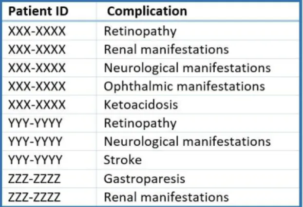
To prepare the data, we needed to perform several steps such as merging tables, creating new variables, and changing the structure of the data tables. In the final dataset, we needed a patient
30
identifier and a complication in each row. Therefore, patients with multiple co-existing
complications had multiple records in the final dataset. Figure 3.1 shows the structure of the final dataset used for the association analysis.
Figure 3.1- Final dataset structure
3.2. Results
In this section, we first present the results of the comorbidity index analysis in different demographic groups of patients. Following that, we compare the prevalence of major diabetes complications in different demographic groups. Finally, we represent the results of the association analysis among diabetes complications.
Comorbidity Index Analysis
In this study, we calculated what we have termed comorbidity index, which is the mean number of complications. The overall index value for the study population was 1.53. Because of the large proportion of diabetic patients with hypertension, we excluded it from our analysis, therefore, the inclusion of hypertension and diabetes itself increases the index value by 2 points to 3.53. Table 3.4 shows index values and descriptive statistics for the racial/ethnic groups examined in this study.
31
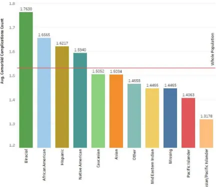
Table 3.4-Comorbidity index value by race/ethnicity
Race/Ethnicity Num. of
Observations Percentage Mean Maximum
Lower 95% CI Upper 95% CI Whole Population 492025 100% 1.53 11 1.529 1.535 Biracial 557 0.11% 1.76 9 1.667 1.859 African American 101582 20.65% 1.66 10 1.650 1.663 Hispanic 7434 1.51% 1.62 8 1.598 1.646 Native American 5394 1.10% 1.59 8 1.567 1.621 Caucasian 302801 61.54% 1.51 11 1.502 1.509 Asian 7145 1.45% 1.50 7 1.482 1.525 Other 14207 2.89% 1.47 9 1.451 1.481
Middle Eastern Indian 103 0.02% 1.45 6 1.281 1.612
Pacific Islander 443 0.09% 1.41 5 1.329 1.484
Asian/Pacific Islander 129 0.03% 1.32 3 1.211 1.424
Missing 52230 10.62% 1.45 8 1.439 1.454
As can be seen in Table 3.4 and Figure 3.2, biracial patients had highest index value with an average of 1.76 complications. African American, Hispanic, and Native American patients all had index values above the population average. Asian/Pacific Islander patients had the lowest index value at 1.32.
32
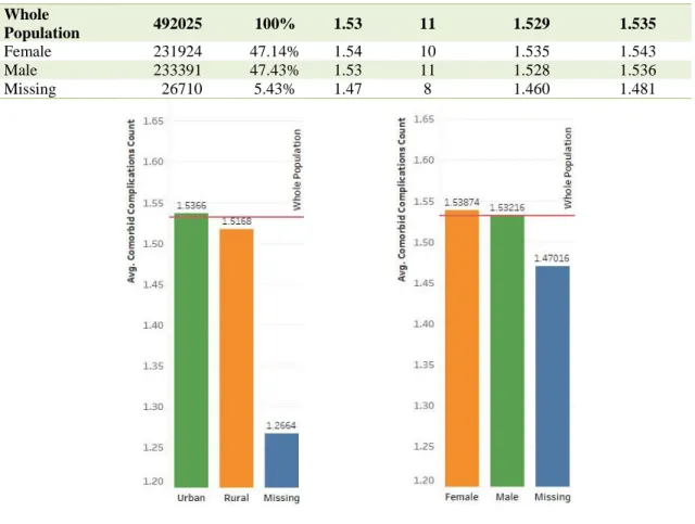
Table 3.5- Comorbidity index value in rural vs urban diabetic patients Urban/Rural
Status
Num. of
Observations Percentage Mean Maximum
Lower 95% CI Upper 95% CI Whole Population 492025 100% 1.53 11 1.529 1.535 Rural 99628 20.25% 1.52 11 1.511 1.523 Urban 391087 79.49% 1.54 10 1.534 1.540 Missing 1310 0.27% 1.27 5 1.241 1.292
Table 3.5 and Figure 3.3a depict the comorbidity index of rural and urban diabetics. Urban patients had slightly higher number of co-exiting complications and this difference was statistically meaningful at the level of 95%. Comorbidity index was not statistically different between males and females as is demonstrated in Table 3.6 and Figure 3.3b.
Table 3.6-Comorbidity index value by gender
Gender Num. of
Observations Percentage Mean Maximum
Lower 95% CI Upper 95% CI Whole Population 492025 100% 1.53 11 1.529 1.535 Female 231924 47.14% 1.54 10 1.535 1.543 Male 233391 47.43% 1.53 11 1.528 1.536 Missing 26710 5.43% 1.47 8 1.460 1.481
Figure 3.3a Figure 3.3b
Figure 3.3a- Comorbidity index value in rural vs urban diabetic patients Figure 3.3b- Comorbidity index value by gender
33
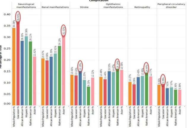
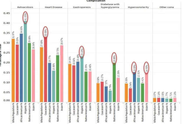
Diabetes Complications Prevalence in Different Demographic Groups
In this section, we compare the prevalence of major diabetes complication by demographic groups. Figures 3.4a and 3.4b demonstrate the racial/ethnic prevalence of complications. Caucasians had the highest prevalence of neurological manifestations and heart disease, while renal manifestations were highest among Asians. Strokes were more prevalent among African Americans, and Native Americans suffered from the highest rates of ophthalmic manifestations, retinopathy, and hyperglycemia. Ketoacidosis and gastroparesis were most common in Hispanics, and hyperosmolarity was more prevalent in African American and Asian patients than other races.