Latent Variable Model for Weight Gain Prevention Data with Informative Intermittent Missingness

Volume 15 | Issue 2 Article 36

11-1-2016

Latent Variable Model for Weight Gain Prevention

Data with Informative Intermittent Missingness

Li Qin

Yale University, [email protected]

Lisa Weissfeld

University of Pittsburgh

Michele Levine

University of Pittsburgh

Marsha Marcus

University of Pittsburgh

Feng Dai

Yale University

Follow this and additional works at:http://digitalcommons.wayne.edu/jmasm

Part of theApplied Statistics Commons,Social and Behavioral Sciences Commons, and the

Statistical Theory Commons

Recommended Citation

Qin, Li; Weissfeld, Lisa; Levine, Michele; Marcus, Marsha; and Dai, Feng (2016) "Latent Variable Model for Weight Gain Prevention Data with Informative Intermittent Missingness,"Journal of Modern Applied Statistical Methods: Vol. 15: Iss. 2, Article 36.

DOI: 10.22237/jmasm/1478003640

Dr. Qin is an Associate Research Scientist of Medicine (Cardiology) in the School of Public Health. Email her at [email protected].

Latent Variable Model for Weight Gain

Prevention Data with Informative Intermittent

Missingness

Li Qin Yale University New Haven, CT Lisa Weissfeld University of Pittsburgh Pittsburgh, PA Michele Levine University of Pittsburgh Pittsburgh, PA Marsha Marcus University of Pittsburgh Pittsburgh, PA Feng Dai Yale University New Haven, CT

Missing data is a common problem in longitudinal studies because of the characteristics of repeated measurements. Herein is proposed a latent variable model for nonignorable intermittent missing data in which the latent variables are used as random effects in modeling and link longitudinal responses and missingness process. In this methodology, the latent variables are assumed to be normally distributed with zero-mean, and the values of variance-covariance are calculated through maximum likelihood estimations. Parameter estimates and standard errors of the proposed method are compared with the mixed model and the complete-case analysis in the simulations and the application to the weight gain prevention among women (WGPW) data set. In the simulation results with respect to bias, mean squared error, and coverage of confidence interval, the proposed model performs better than the other two methods in different scenarios. Relatively, the proposed latent variable model and the mixed model do a better job for between-subject effects compared to within-subject effects. The converse is true for the complete case analysis. The simulation results also provide support for application of this proposed latent variable model to the WGPW data set.

Keywords: Latent variable, longitudinal study, non-ignorable missing data, weight gain prevention

Introduction

Missing data is a common issue encountered in the analysis of longitudinal data. In the behavioral intervention setting, missed visits and/or losing to follow up can be extremely problematic. In this area, missed visits are assumed to be a result of

failure of the intervention, sustained lack of interest in the study, or decreased desire to change the behavior (Qin et al., 2009). For weight loss studies, these are common issues that must be dealt with at the data analysis phase. For example, Levine et al. (2007) conducted a weight gain prevention study among women (WGPW) aged 25 to 45 years old. Participants were assessed for BMI (Body Mass Index) at baseline, year one, two and three. However, the outcomes at follow-ups for some women were missing. Because the missing data might be related to their unobserved BMIs, they were considered as nonignorable, informative, or missing not at random (MNAR) (Rubin, 1976).

To account for informative missingness, a number of model-based approaches were proposed to jointly model the longitudinal outcome and the missingness mechanism. The methodology adopted here is motivated by latent pattern mixture models (Lin, McCulloch, & Rosenheck, 2004) and latent dropout class models (Roy, 2003). In latent pattern mixture models, the mixture patterns are formed from latent classes that link the longitudinal responses and the missingness process. A non-iterative approach has been proposed, to assess the assumption of the conditional independence between the longitudinal outcomes and the missingness process given the latent classes (Lin et al., 2004). Roy (2003) noted the idea of pattern-mixture models (e.g., Little, 1993) is not appropriate in many circumstances, because there are many reasons for missingness and subjects with the same missingness pattern may not share a common distribution. Roy (2003) assumed the existence of a small number of dropout classes behind the observed dropout times. But for Roy (2003)’s method, it is difficult to decide the number of latent classes ahead of the analysis. It also leads to misclassification because it is difficult to divide subjects into classes due to the variety of reasons for missingness. Some subjects may not belong to any latent classes. So it is reasonable and straightforward to propose a latent variable model in which the latent variable is unobserved and continuous.

The WGPW study data (Levine et al., 2007) provides motivation to adopt the latent pattern mixture model methodology. In this trial, interventions were compared with a control group in preventing weight gain among normal or overweight women. 190 women were randomized to clinic-based group intervention and information-only control condition. For women randomized to the interventions, treatment was provided over a two-year period, with a follow-up at year three. All women participated in yearly assessment. The primary outcome of interest was body mass index (BMI) calculated from weight assessed yearly and height at baseline. Overall, 81%, 76% and 36% completed a weight assessment at year one, two and three, respectively. The reasons for this

incompleteness may be related to their unobserved outcomes. To avoid biased estimations, possible dependence of missingness status on unobserved responses has to be considered.

A latent variable model is proposed for informative intermittent missingness, developed from Henderson, Diggle, and Dobson’s (2000) joint modeling of longitudinal measurements and event time data. In the proposed model, longitudinal process and missing data process are linked through a latent bivariate Gaussian process W(t) = {W1(t), W2(t)}. An assumption of this latent variable model is that the longitudinal measurements and missing data process are conditional independent given W(t). This assumption simplifies likelihood function. It also increases the strength of the relationship between the missing data process and underlying true outcome process determined by the correlation between W1(t) and W2(t).

The proposed latent variable model and the parameter estimation is described in next section. A simulation study is carried out in the following section, to compare the performance of the latent variable model with mixed model and complete-case analysis. The proposed model is then applied to the WGPW data (Levine et al., 2007) and compared with the mixed model and complete-case analysis, and the assessment of fit of the model is treated. A discussion is provided in the last section.

Model specification and estimation

Assume the proposed latent variable model is present for the full data. Denoting a normally distributed continuous response variable measured on the ith _{subject at}

the jth _{occasion as Y}

ij (i = 1, …, N; j = 1, …, K), the K intended responses are collected into a vector Yi = (Yi1, …, YiK) if there is no missing data.

For various reasons, not all subjects have all K measurements. Here the baseline measure Yi1 is assumed to be observed for every individual. When

missingness process occurs as a result of dropout, the response Yij for subject i is only observed at time points j = 1, …, ki; where ki ≤ K. But if the data are subject to intermittent missingness, before time point ki, there may be additional missing measurements. A missingness indicator, Rij, is used for each of the K measurements, with 1 if Yij is missing and 0 if Yij is observed.

In the following, random-effect models are briefly described for the separate analysis of longitudinal data and missingness procedure, and the joint model via a latent zero-mean bivariate Gaussian process.

Longitudinal Responses

The sequence of longitudinal measurements Yi1, Yi2, …, YiK for the ith subject at times ti1, ti2, …, tiK is modeled as

Yij = βTxij + W1i (tij) + εij, where βT_x

ij = μij is the mean response in which the vector β and xij represent possibly time-varying explanatory variables and their corresponding regression coefficients, respectively; W1i(tij) incorporates subject-specific random effects; and εij ~ N(0, σε2) is a sequence of mutually independent measurement errors corresponding to Yij. The W1i(tij) can be viewed as the actual individual variability of outcome trajectories after they have been adjusted for the overall mean trajectory and other fixed effects.

Missing Data Procedures

Here Rij = 1 is defined as Yij being missing, and Rij = 0 as Yij being observed. Letting φij denote the probability of Rij = 1, the logistic model for φij is specified as

log

j

ij 1-

j

_ij = α

T_z

ij + W2i (tij).

where α is a vector of log odds ratios corresponding to zij; zij is a vector of covariates specific to the missingness process for subject i; and W2i(tij) represents random effect.

Latent Variable Model

The dependence between the missingness process and longitudinal responses is characterized by sharing a common random effect vector for the ith _{subject, say}

(W1i, W2i)T, which is independent across different subjects. Thus, the stochastic dependence between W1i and W2i is critical. It is referred as latent association. Before specifying (W1i, W2i)T, the pair of latent variables (U1i, U2i)T are defined with a mean-zero bivariate Gaussian distribution N(0, Σ) (Henderson et al., 2000). The (W1i, W2i)T are then modeled as

W_2i (t) = λ₁U_1i + λ₂U_2it

Both W1i andW2i are represented as random intercept and slope terms; s and t are possibly time-varying explanatory variables; λ1 and λ2 are the parameters measuring the association between W1i andW2i, that is, the association between longitudinal and missing data processes induced through the intercept, slope and current W1 value. The derivatives of W2i are as follows:

W_2i (t) = λ₁U_1i + λ₂U_2it

= γ₁U_1i + γ₂U_2it + γ₃(U_1i + U_2it) = γ₁U_1i + γ₂U_2it + γ₃W_1i (t), where λ1 = γ1 + γ3 and λ2 = γ2 + γ3.

In this way, the traditional Laird-Ware random effects models are combined with a proportionality assumption W2i(t) ∝ W1i(t). A simple case of this assumption is W2i(t) = W1i(t), in which γ1 = γ2 = 0 and γ3 = 1. The proportionality assumption allows us to consider more complicated situations in which the association between longitudinal and missing data processes is described in terms of the intercept and slope. In other words, the impact of underlying random effect structure differences between the longitudinal and missing data processes can be assessed. The fixed effects in sub-models mentioned earlier in this section, xij and

zij, may or may not correspond to the same covariates. Actually, the dependence between Yij and φij may arise in two ways: through the common fixed effects or through stochastic dependence between W1i and W2i. Even if W1i and W2i are independent, the longitudinal and missing data processes still could be associated through the common fixed effects.

Estimation

Let yi, yic _{and yi}m _{denote the vector of observed, complete and missing} longitudinal responses for the ith _{subject. Let ψ}T _{= (β}T_{, α}T_{, γ}T_{) represent the set of}

parameters of interests; the observed log-likelihood for the joint model is

logL

(

y;y,j,W|x,z

)

=

ò

_ëélogL

(

b;y_ic|x_i,j_i,W_i

)

+logL

(

a;j_i|z_i,W_i

)

+logL

( )

g;W_i ù_ûdy_im

i=1

N

å

= éëlogL

(

b;y_i|x_i,W_i

)

+logL

(

a;j_i|z_i,W_i

)

+logL

( )

g;W_i ùû

i=1

N

å

logL

(

b

;y_i|x_i,W_i

)

= - 1 2

( )

log 2

( )

p +log se 2+ S 11

(

)

+ s_e2+ S 11

(

)

-1 y_i-bT_x i-W1i

(

)

T y_i-bT_x i-W1i

(

)

é ë ê ê ù û ú ú, logL

(

a

;

j

_i|z_i,W_i

)

= R_ij j=1 K

å

log

j

_ij = R_ij j=1 K

å

a

T_z ij+W2i

(

)

-log exp

(

a

Tz_ij+W_2i

)

j=1 K

å

ì í îï ü ý þï, logL

( )

g

;W_i = - 1 2

( )

élog 2

( )

p

2+logS +

(

W_i-

m

_i

)

TS-1

(

W_i-

m

_i

)

ëê ùûú.

m

_i = U1i+U2is

l

₁U_1i+

l

₂U_2it æ è ç ç ö ø ÷ ÷

is the mean vector for Wi. Here let

logL

(

b

;y_i|x_i,

j

_i,W_i

)

=logL

(

b

;y_i|x_i,W_i

)

,

that is, given the latent variables Wi, the outcome Yi is independent of the missingness φi. This is an important assumption which reduces the mathematical complexity for estimation. Because φi affects yi through Wi, the missingness is not ignored in the maximum likelihood inference.

The maximum likelihood estimation of the joint model is obtained by the quasi-Newton method, in which the latent variables are estimated by empirical Bayes and standard errors are estimated using the delta method. Because the likelihood equations for the L(α;φi | zi,Wi) are non-linear (from logistic regression) and do not have closed form maximizers, which may lead to some maximization algorithms having difficulty converging, a modified quasi-Newton algorithm is used for maximizing the likelihood. For example, the current estimate of ψ is updated by

y

( )k+1 =

y

( )k -

a

( )k ¶ 2_l

( )

y

¶

y

¶

y

T ì í ï îï ü ý ï þï -1 ¶l

( )

y

¶

y

where l(ψ) = logL(ψ; y,φ,W | x,z), and a(k) is a small constant with values between 0 and 1. Generally, a(k) starts from very small (e.g., 0.01) toward 1 as k

to make sure that it will converge to a global maximum. Here, the starting values are chosen from the estimates of complete-case analysis.

Sensitivity Analysis

The proposed method assumes that the distribution of the longitudinal responses (both observed and missing) does not depend on the missingness procedure after conditioning to latent zero-mean bivariate Gaussian process. This conditional independence assumption is strong, and neither it nor the missing not at random assumption can be tested just using the observed data. The sensitivity analyses will be considered for these assumptions by comparing the new model with commonly used mixed model and complete-case analysis in the simulation and data analysis sections. Results by the proposed method will be reported with different latent processes W1(s) and W2(t). Akaike’s information criterion (AIC)

(Akaike, 1981) and the Bayesian information criteria (BIC) (Schwartz, 1978) will be used to assess model fit. It must be kept in mind that the unobserved outcomes cannot be checked in any sensitivity analyses.

Simulation study

A small simulation study was carried out to compare the performance of the latent variable model with mixed model under MAR assumption and complete-case analysis that discards subjects with missing observations. The data sets were generated by considering two aspects: the complete data structure with outcomes and observable independent variables; and the missingness structure.

Complete data is generated with N = 200 subjects with J = 4 time points. It is assumed that there are 2 treatment groups with an equal number of subjects in each group. The following specifications for the longitudinal component are assumed: intercept = −0.5; treatment (Tx) = 1.0; time 2 vs. time 1 (T2 – T1) = 0.5; time 3 vs. time 1 (T3 – T1) = 1.0; time 4 vs. time 1 (T4 – T1) = 1.5. Consequently the mean of the dependent variable Yij can be written as:

E(Y_ij) = β₀ + β₁Tx + β₂ (T₂ – T₁) + β₃ (T₃ – T₁) + β₄ (T₄ – T₁)

where β0 = −0.5, β1 = 1.0, β2 = 0.5, β3 = 1.0, and β4 = 1.5 as defined above. Tx is the variable for treatment groups with values of 0 or 1; (T2 – T1) = 1 if Yij is observed at time point 2, 0 otherwise; (T3 – T1) and (T4 – T1) are defined similarly with a value of 1 if Yij is observed at time point 3 or 4 and a value of 0 otherwise.

The error term of outcomes Yi follows a compound symmetry structure, with variance 1 and covariance 0.5.

For missingness component, the assumption of missing not at random (MNAR) will be followed directly: that is, the missingness depends on the unobserved variables. Here let missingness procedure follow a logistic regression with an intercept and current unobserved response as the only covariate. Specifications are assumed as: intercept (α0) = −3.0 and log odds ratio for the current unobserved response (α1) = 1.5, 1.0 or 0.5. That is:

log

j

ij

1-

j

_ij =

a

0+

a

1yij.

The summary measures for a parameter estimate include: a) mean bias: the mean difference of a sample estimate from the true parameter average over iterations of a simulation run; b) mean squared error: the mean of the squared deviation of a sample estimate from the true parameter averaged over iterations of a simulation run; and c) the coverage of nominal 95% confidence intervals, obtained by computing the percentage of iterations for which the corresponding nominal 95% confidence interval included the true parameter (Ten Have, Kunselman, Pulkstenis, & Landis, 1998). Data are generated 1000 times under each scenario for the proposed model (latent variable model, LVM), a mixed model (MM) for all available data, and a mixed model that discards the missed observations, that is, a complete-case analysis (CC).

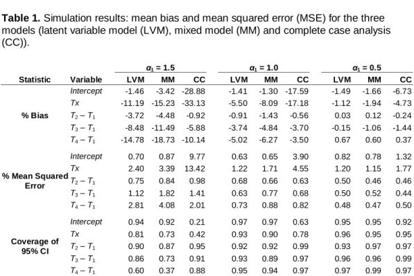
The simulation results are presented in Table 1. When missingness strongly depends on the unobserved outcomes (α1 = 1.5), the time effects (T2 – T1, T3 – T1, and T4 – T1) are underestimated (negative bias) and coverage of 95% confidence interval is poor under the mixed model. For complete-case analysis, the between-subject effect (Intercept and Tx) estimates and confidence interval coverage do not exhibit good properties, though the mixed model displays just the opposite, that is, it is accurate in the between-subject effect estimates but not in the within-subject effect (time effect) estimates. For the proposed method, both within- and between-subject inference are accurate even under the strong dependence on the unobserved outcomes except for the effect of (T4 – T1), which is due to the small number of observations at T4.

Table 1. Simulation results: mean bias and mean squared error (MSE) for the three models (latent variable model (LVM), mixed model (MM) and complete case analysis (CC)). α1 = 1.5 α1 = 1.0 α1 = 0.5 Statistic Variable LVM MM CC LVM MM CC LVM MM CC % Bias Intercept -1.46 -3.42 -28.88 -1.41 -1.30 -17.59 -1.49 -1.66 -6.73 Tx -11.19 -15.23 -33.13 -5.50 -8.09 -17.18 -1.12 -1.94 -4.73 T2 – T1 -3.72 -4.48 -0.92 -0.91 -1.43 -0.56 0.03 0.12 -0.24 T3 – T1 -8.48 -11.49 -5.88 -3.74 -4.84 -3.70 -0.15 -1.06 -1.44 T4 – T1 -14.78 -18.73 -10.14 -5.02 -6.27 -3.50 0.67 0.60 0.37 % Mean Squared Error Intercept 0.70 0.87 9.77 0.63 0.65 3.90 0.82 0.78 1.32 Tx 2.40 3.39 13.42 1.22 1.71 4.55 1.20 1.15 1.77 T2 – T1 0.75 0.84 0.98 0.68 0.66 0.63 0.50 0.46 0.46 T3 – T1 1.12 1.82 1.41 0.63 0.77 0.68 0.50 0.52 0.44 T4 – T1 2.81 4.08 2.01 0.73 0.88 0.82 0.48 0.47 0.50 Coverage of 95% CI Intercept 0.94 0.92 0.21 0.97 0.97 0.63 0.95 0.95 0.92 Tx 0.81 0.73 0.42 0.93 0.90 0.78 0.96 0.95 0.95 T2 – T1 0.90 0.87 0.95 0.92 0.92 0.99 0.93 0.97 0.97 T3 – T1 0.86 0.73 0.91 0.93 0.89 0.97 0.96 0.96 0.99 T4 – T1 0.60 0.37 0.88 0.95 0.94 0.97 0.97 0.99 0.97

Application to WGPW data

Data description and model specifications

The proposed latent variable model is applied to an actual data set to illustrate its features and explore issues involved with its implementation. The sensitivity of inference to the model assumption and constraints in model formulation are also considered.

To illustrate the method, a subset of data from a study involving weight gain prevention in women (WGPW) is used. This trial was conducted in the Department of Psychiatry at the University of Pittsburgh Medical Center (Levine et al., 2007), and involved 25- to 45-year-old women at risk for weight gain and future obesity. The primary aim of the trial was to compare the relative efficacy of three approaches to weight gain prevention: a clinic-based group intervention, a mailed, correspondence intervention and an information-only control group. The measurements were taken at baseline, year 1, year 2 and year 3.

For the analysis, 190 women with complete baseline data are focused on and randomized into the clinic-based group and the control group. Women randomized to the clinic-based intervention group were required to attend 15

group meetings over a 24-month period. These sessions were held biweekly for the first 2 months and bimonthly for the next 22 months. Biweekly sessions focused on self-monitoring of energy intake and expenditure, and behavioral strategies for making modest changes in dietary intake and activity level. During the 11 bimonthly clinic-based meetings, participants received lessons on cognitive change strategies, stimulus control techniques, problem solving, goal setting, stress and time management, and relapse prevention. Women belonging to the control group received booklets containing information about the benefits of weight maintenance, low-fat eating, and regular physical activity.

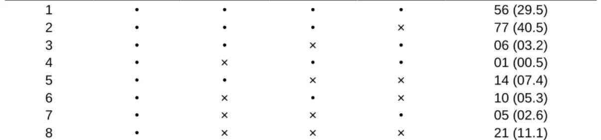
About 70% of the women did not complete their scheduled assessments (Table 2). It was suspected that this was in part due to reasons related to their weight outcomes. Among women randomized to the intervention group in which treatment was provided over a 2-year period, 20% missed the weight assessments at year 1; 27% at year 2; and 63% at year 3 of the follow-up. For subjects in the control group, 19%, 22% and 66% missed the weight assessments at year 1, 2 and 3. The plot in Figure 1 indicates that at year 2, which is the end of the treatment, the intervention group exhibits a lower BMI than the control group. However the plot of Figure 2 indicates that at year 2, the probability of missingness in the intervention group is a little higher than that of the control group. If only the observed data are used, the conclusion that the intervention group has a smaller BMI at the end of the treatment (year 2) may be reached. But if the missing data mechanism is considered, what will the data tell us?

Table 2. Distribution of the missingness patterns for WPGW data.

Pattern Baseline Year 1 Year 2 Year 3 Frequency (%)

1 • • • • 56 (29.5) 2 • • • × 77 (40.5) 3 • • × • 06 (03.2) 4 • × • • 01 (00.5) 5 • • × × 14 (07.4) 6 • × • × 10 (05.3) 7 • × × • 05 (02.6) 8 • × × × 21 (11.1)

Figure 1. Observed BMI mean (SE) across years for each treatment group

Let Yij denote the BMI measurement on the ith patient at the jth year in the trial, j = 0, 1, 2 and 3. Six explanatory variables are included as main effects in the analysis: treatment (Tx, intervention = 1 and control = 0), years in the trial (year), patient age when enrolled (age), dietary restraint (S3FS1, range from 0–21), disinhibition (S3FS2, range from 0–16), and perceived hunger (S3FS3, range from 0–14). Among them, dietary restraint, disinhibition and perceived hunger belong to Stunkard Three-Factor Eating Questionnaire, and they are included in the model as time-variant predictors, as is year. The linear random effects model for BMI is specified as

Y_ij = β₀ + β₁year_j + β₂year_j

× Tx_i + β₃age_i + β₄S3FS1_ij + β₅S3FS2_ij + β₆S3FS3_ij + W_1i(year_j), where W_1i(year_j) is the random effect.

Similarly the missingness procedure is modelled with the logistic regression with random effect, W2i(yearj). Let φij = Pr(Yij is missing),





0 1 2 log 1 ij i i j ij Tx W year         .

To choose the exact forms of W1i and W2i, Akaike’s information criterion (AIC) (Akaike, 1981) and the Bayesian information criterion (BIC) (Schwartz, 1978) are used. The results are given in Table 3: because Model VII emerges with the smallest values of AIC and BIC, it is selected over the others, and also demonstrates the full complexity of (W1i, W2i)T given under the Latent Variable Model, earlier. In Model VII, W1i(yearj) = U1i + U2iyearj. So W1i(yearj) includes

random effects for intercept and slope over time, where



1, 2



~ 2

 

0,

iid T

i i i

U  U U N  and variance-covariance structure

11 12 12 22         _{ }    .

This structure of random effects allow that each subject has her own baseline BMI value and time trend of BMIs over years in the trial. And the random effects in the

models of missingness procedure are chosen as

W2i(yearj) = r1U1i + r2U2iyearj + r3(U1i + U2iyearj), where U1i and U2i are defined as before. In the following application results and interpretations, inferences will be based on these chosen random effect structures.

Table 3. Descriptive of model fit for different random effect structures for WGPW data.

Model W1i W2i

−2 log

likelihood AIC BIC

I 0 0 2904.4 2936.4 3018.0 II U1i 0 2656.6 2657.6 2709.6 III U1i γ1U1i 2625.3 2657.3 2709.3 IV U1i+ U2iyearj 0 2595.9 2629.7 2679.8 V U1i+ U2iyearj γ1U1i 2595.7 2627.7 2679.6 VI U1i+ U2iyearj γ1U1i+ γ2U2i 2614.6 2656.6 2698.6 VII U1i+ U2iyearj γ1U1i+ γ2U2i+ γ3W1i 2534.7 2566.7 2618.6 Model interpretation

Table 4 details the model estimates of treatment, time, age, dietary restraint, disinhibition and perceived hunger effects on the BMIs. In Table 5, the estimates in the missingness component of the joint model are compared to the analogous estimates from a random effects model, which ignores the BMI outcome, to address the effects of treatment on the missingness status. In both tables, the estimates for variance-covariance structure Σ under models for longitudinal responses and missing data procedure, separately and jointly, are discussed.

As shown in Table 4, the mixed model, under the assumption of missing at random, and the proposed joint model yield similar inference for significant effect of year, whereas the complete case analysis under the assumption of missing completely at random does not show any significant time effect. In the proposed model, age effect intends to be significant (p value = 0.074), although in the other two models, there is no such intention. Under all three models, dietary restraint and disinhibition show strong effects (p values < .0001). In Table 5, the association parameter in the proposed method, γ3, is negative and significantly different from zero. It provides a strong evidence of association between the two sub-models of the proposed method, and indicates that the slope of observed BMI values is negatively associated with the missingness status, because of

λ2 = γ2 + γ3 < 0 with γ2 = 6.779 and γ3 = −26.94 (Table 5). This may result from patients with larger BMI values having lower probabilities of dropping out, leaving their relatively larger BMI values in the trial.

Comparisons with simulation results

The relationship between the proposed method and the mixed model in the application to the WGPW data is now checked, and compared with the patterns observed in the simulations. Table 4 reveals that the proposed method and the

mixed model yield similar between-subject effect estimates (age, dietary restraint, disinhibition and perceived hunger), but are different in the within-subject inference (year, and year × treatment). As in the simulation results, the mixed model gives accurate inference in between-subject effect estimates but not in within-subject effect estimates. This congruence in the between-subject effect estimates, and difference in the within-subject effect estimates, provides evidence that the proposed method is a good choice for the WGPW data.

Table 4. Parameter estimates, estimated standard errors and p-values for modeling the outcomes, BMI.

CC analysis Mixed Model Latent Variable model

Variable Estimate SE p-value Estimate SE p-value Estimate SE p-value

Intercept 24.3000 2.1350 <0.0001 22.8200 1.1410 <0.0001 22.8400 1.1590 <0.0001 Year 0.0770 0.1400 0.5850 0.2030 0.0920 0.0290 0.1520 0.0750 0.0440 Year × Treatment -0.0240 0.1920 0.9030 -0.1630 0.1280 0.2020 -0.1240 0.1030 0.2300 Age 0.0370 0.0580 0.5250 0.0470 0.0300 0.1180 0.0550 0.0300 0.0740 Dietary Restraint -0.2090 0.0370 <0.0001 -0.1200 0.0220 <0.0001 -0.1320 0.0240 <0.0001 Disinhibition 0.1650 0.0520 0.0030 0.1800 0.0320 <0.0001 0.1780 0.0330 <0.0001 Perceived Hunger -0.0270 0.0450 0.5460 -0.0180 0.0300 0.5610 -0.0280 0.0320 0.3940 Σ11 1.9480 0.2300 <0.0001 2.0180 0.1300 <0.0001 2.0490 0.1250 <0.0001 Σ12 -0.0090 0.1120 0.9370 -0.0230 0.0750 0.7620 0.0040 0.0090 0.6720 Σ22 0.4940 0.0940 <0.0001 0.5280 0.0690 <0.0001 0.0620 0.0410 0.1300 σε2 0.9400 0.0720 <0.0001 0.8620 0.0500 <0.0001 1.0680 0.0460 <0.0001

Table 5. Parameter estimates, estimated standard errors and p-values for modeling the missingness status, R.

Separate Analysis Latent Variable Model

Variable Estimate SE p-value Estimate SE p-value

Intercept -1.0620 0.1350 <0.0001 -2.5910 0.3580 <0.0001 Treatment 0.0360 0.1800 0.8410 0.0700 0.3320 0.8320 γ1 NA NA NA 27.0600 17.9600 0.2400 γ2 NA NA NA 6.7790 5.7500 0.1360 γ3 NA NA NA -26.9400 17.9700 <0.0001

Conclusion

A latent variable model was proposed to fit longitudinal data with informative intermittent missingness. The main idea is to jointly model the longitudinal process and missing data process via a latent zero-mean bivariate Gaussian

process on (W1(t), W2(t))T_{, with correlation between W1(t) and W2(t), inducing} stochastic dependence between the longitudinal and missing data processes. An advantage of this method, compared with other existing methods for informative missing data problems, is its easy implementation. The models in this method can be easily fit after providing the likelihood functions. Thus it avoids the complexity of EM algorithm programming, facilitating use of this proposed method in practice. The specifications and selections of W1(t) and W2(t) can be implemented via AIC and BIC, and the method enables direct comparisons of different specifications.

In the proposed method, the latent variables are also used to induce conditional independence between the responses (both observed and missing) and missingness status, so that the standard likelihood techniques can be used to derive the estimates. This is a strong assumption and it cannot be tested with the available data. For this type of assumption, a sensitivity analysis is the way to investigate the model fit and departure of the assumption. Such an analysis has been attempted by comparing the proposed method with other alternative models in the true data and in simulations.

The proposed method is developed from the joint model proposed by Henderson et al. (2000) for longitudinal and survival processes. In the future, this method should be considered for extension into other applications, through different link functions (e.g. binary or ordinal data) or random effect structures other than zero-mean bivariate Gaussian distribution.

References

Akaike, H. (1981). Likelihood of a model and information criteria. Journal of Econometrics,16(1), 3-14. doi: 10.1016/0304-4076(81)90071-3

Henderson, R., Diggle, P. J. & Dobson, A. (2000). Joint modeling of

longitudinal measurements and event time Data. Biostatistic,s1(4), 465–480. doi:

10.1093/biostatistics/1.4.465

Levine, M. D., Klem, M. L., Kalarchian, M. A., Wing, R. R., Weissfeld, L., Qin. L. & Marcus. M. D. (2007). Weight gain prevention among women. Obesity, 15(5), 1267-1277. doi: 10.1038/oby.2007.148

Lin, H., McCulloch, C. E. & Rosenheck, R. A. (2004). Latent pattern mixture models for informative intermittent missing data in longitudinal studies.

Little, R. J. A. (1993). Pattern-mixture models for multivariate incomplete data. Journal of the American Statistical Association,88(421), 125–134. doi:

10.1080/01621459.1993.10594302

Qin, L., Weissfeld, L. A., Shen, C. & Levine, M. D. (2009). A two-latent-class model for smoking cessation data with informative dropouts.

Communications in Statistics – Theory and Methods,38(15), 2604 - 19. doi:

10.1080/03610920802585849

Roy, J. (2003). Modeling longitudinal data with nonignorable dropouts using a latent dropout class model. Biometrics,59(4), 829–836. doi:

10.1111/j.0006-341X.2003.00097.x

Rubin, D. B. (1976). Inference and missing data. Biometrika,63(3), 581– 590. doi: 10.1093/biomet/63.3.581

Schwartz, G. (1978). Estimating the dimension of a model. Annals of Statistics,6(2), 461-464. doi: 10.1214%2Faos%2F1176344136

Ten Have, T. R., Kunselman, A. R., Pulkstenis, E. P. & Landis, J. R. (1998). Mixed effects logistic regression models for longitudinal binary response data with informative dropout. Biometrics,54(1), 367–383. doi: 10.2307/2534023