Margin Trees for High-dimensional Classification
Robert Tibshirani [email protected]
Trevor Hastie [email protected]
Departments of Health, Research & Policy, and Statistics Stanford University
Stanford, CA 94305
Editor: Dale Schurmanns
Abstract
We propose a method for the classification of more than two classes, from high-dimensional fea-tures. Our approach is to build a binary decision tree in a top-down manner, using the optimal margin classifier at each split. We implement an exact greedy algorithm for this task, and compare its performance to less greedy procedures based on clustering of the matrix of pairwise margins. We compare the performance of the “margin tree” to the closely related “all-pairs” (one versus one) support vector machine, and nearest centroids on a number of cancer microarray data sets. We also develop a simple method for feature selection. We find that the margin tree has accuracy that is competitive with other methods and offers additional interpretability in its putative grouping of the classes.
Keywords: maximum margin classifier, support vector machine, decision tree, CART
1. Introduction
We consider the problem of classifying objects into two or more classes, from a set of features. Our main application area is the classification of cancer patient samples from gene expression measure-ments.
When the number of classes K is greater than two, maximum margin classifiers do not gen-eralize easily. Various approaches have been suggested, some based on the two-class classifier (“one-versus-all” and “one-versus one’ or “all pairs’), and others modifying the support vector loss function to deal directly with more than two classes (Weston and Watkins, 1999; Lee et al., 2004; Rosset et al., 2005). These latter proposals have a nice generalization of the maximum margin property of the two class support vector classifier. Statnikov et al. (2004) contains a comparison of different support vector approaches to classification from microarray gene expression cancer data sets. While these methods can produce accurate predictions, they lack interpretability. In particular, with a large number of classes, the investigator may want not only a classifier but also a meaningful organization of the classes.
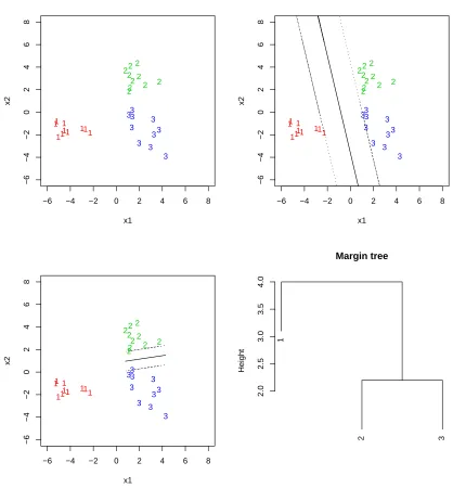
The best line is shown in the top right panel, splitting class 1 from classes 2 and 3. We then focus just on classes 2 and 3, and their maximum margin classifier is shown in the bottom left. The overall top-down classifier is summarized by the binary tree shown in the bottom right panel.
We employ strategies like this for larger numbers of classes, producing a binary decision tree with a maximum margin classifier at each junction in the tree.
In Section 2 we give details of the margin tree classifier. Section 3 shows the application of the margin tree to a number of cancer microarray data sets. For construction of the tree, all of the classifiers in the margin tree use all of the features (genes). In Section 4 we discuss approaches to feature selection. Finally in Section 5 we have some further comments and a discussion of related work in the literature.
2. The Margin Tree Classifier
Denote the gene expression profiles by xj = (x1 j,x2 j, . . .xp j)for j=1,2, . . .N samples falling into
one of K classes. The features (genes) are indexed by i=1,2, . . .p.
Consider first the case of K =2 classes, C1 and C2. The class outcome is denoted by yj =
±1. The maximum margin classifier is defined by the constantβ0 and the weight vectorβ with components∑iβ2i =1 that maximizes the gap between the classes, or the “margin”. Formally,
(β0,β) = argmax(C)
where yj(β0+
∑
iβixi j)≥C ∀j.
The achieved margin M=2·C. In the examples of this paper, p>N so that all classes are separable and M>0. We have some discussion of the non-separable case in Section 5.
Now suppose we have K>2 classes. We consider three different strategies for constructing the tree. These use different criteria for deciding on the best partition of the classes into two groups at each juncture. Having settled on the partition, we use the maximum margin classifier between the two groups of classes, for future predictions.
Let M(j,k) be the maximum margin between classes j and k. Also, let G1,G2 be groups of classes, and let M(G1,G2)denote the maximum margin between the groups. That is, M(G1,G2)is the maximum margin between two hyper-classes: all classes in G1and all classes in G2. Finally, denote a partition by P={G1,G2}.
Then we consider three approaches for splitting a node in the decision tree:
(a) Greedy: maximize M(G1,G2)over all partitions P.
(b) Single linkage: Find the partition P yielding the largest margin M0so that min M(j1,j2)≤M0 for j1,j2∈Gk,k=1,2 and min M(j1,j2)≥M for j1∈G1,j2∈G2.
(c) Complete linkage: Find the partition P yielding the largest margin M0so that max M(j1,j2)≤ M0for j1,j2∈Gk,k=1,2 and max M(j1,j2)≥M0for j1∈G1,j2∈G2.
The greedy method finds the partition that maximizes the resulting margin over all possible partitions. Although this may seem prohibitive to compute for a large number of classes, we derive an exact, reasonably fast algorithm for this approach (details below).
−6 −4 −2 0 2 4 6 8 −6 −4 −2 0 2 4 6 8 x1 x2 1 1 1 1 1 1 1 1 1 1 2 2 2 2 2 2 2 2 2 2 3 3 3 3 3 3 3 3 3 3
−6 −4 −2 0 2 4 6 8
−6 −4 −2 0 2 4 6 8 x1 x2 1 1 1 1 1 1 1 1 1 1 2 2 2 2 2 2 2 2 2 2 3 3 3 3 3 3 3 3 3 3
−6 −4 −2 0 2 4 6 8
−6 −4 −2 0 2 4 6 8 x1 x2 1 1 1 1 1 1 1 1 1 1 2 2 2 2 2 2 2 2 2 2 3 3 3 3 3 3 3 3 3 3 1 2 3 2.0 2.5 3.0 3.5 4.0 Margin tree Height
each pair of classes. Single linkage clustering successively merges groups based on the minimum distance between any pair of items in each of the group. Complete linkage clustering does the same, but using the maximum distance. Now having built a clustering tree bottom-up, we can interpret each split in the tree in a top-down manner, and that is how criteria (b) and (c) above were derived. In particular it is easy to see that the single and complete linkage problems are solved by single and complete linkage agglomerative clustering, respectively, applied to the margin matrix M(j1,j2). Note that we are applying single or complete linkage clustering to the classes of objects Cj, while
one usually applies clustering to individual objects.
The greedy method focuses on the form of the final classifier, and tries to optimize that classifi-cation at each stage. Note that the greedy method cares only about the distance between classes in the different partitions, and not about the distance between classes within the same partition. Both the single linkage and complete linkage methods take into account both the between and within partition distances. We will also see in the next section that the complete linkage method can be viewed as an approximation to the greedy search.
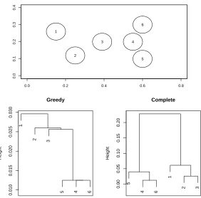
Figure 2 shows a toy example that illustrates the difference between the greedy and complete linkage algorithms. There are six classes with circular distributions. The greedy algorithm splits off group 1,2, and 3 in succession, and then splits off 4,5,6 as a group. This is summarized in the bottom left panel. The complete linkage algorithm in the bottom right panel instead groups 1,2 and 3 together and 4,5, and 6 together. The complete linkage tree is more balanced and hence may be more useful biologically.
In the experiments in this paper we find that:
• All three methods produce about the same test set accuracy, and about the same as the all-pairs maximum margin classifier.
• The complete linkage approach gives more balanced trees, that may be more interpretable that those from the other two methods; the single linkage and greedy methods tend to produce long stringy trees that usually split off one class at a time at each branch. The complete linkage method is also considerably faster to compute than the greedy method.
Thus the complete linkage margin tree emerges as our method of choice. It requires computation of
K
2
support vector classifiers for each pair of classes for the complete linkage clustering and then for the final tree, one computation of a support vector classifier for each node in the tree (at most K and typically≈log2(K)classifiers.)
2.1 An Exact Algorithm for the Greedy Criterion
A key fact is
M(G1,G2)≤min{M(j1,j2),j1∈G1,j2∈G2}. (1)
That is, the margin between two groups of classes is less than or equal to the smallest margin between any pair of classes, one chosen from each group.
0.0 0.2 0.4 0.6 0.8
0.0
0.1
0.2
0.3
0.4
1
2
3 4
5 6
1
2 3
5 4 6
0.010
0.015
0.020
0.025
0.030
Height
Greedy
5
4 6
1
2 3
0.00
0.05
0.10
0.15
0.20
Height
Complete
Figure 2: A toy example illustrating the difference between the greedy and complete linkage algo-rithms. There are six classes with circular distributions (top panel). The greedy algorithm splits off groups 1,2, and 3 in succession, and then splits off 4,5,6 as a group. This is sum-marized in the bottom left panel. The complete linkage algorithm (bottom right panel) instead groups 1,2 and 3 together, and 4,5, and 6 together. For example, the margin be-tween classes 1 and 2 is 0.0296, while that bebe-tween 3 and 4 is less: 0.0256. The height in each plot is the margin corresponding to each join.
at least M with every other class in that node. Hence we need only consider partitions that keep the collapsed nodes intact.
We summarize the algorithm below:
Exact computation of the best greedy split
1. Construct the complete linkage clustering tree based on the margin matrix M(j1,j2).
3. Cut the complete linkage tree at height M0, and collapse all nodes at that height.
4. Consider all partitions of all classes that keep the collapsed nodes intact, and choose the one that gives maximal margin ˆM.
This procedure finds the partition of the classes that yields the maximum margin. We then apply this procedure in a top-down recursive manner, until the entire margin tree is grown.
This algorithm is exact in that it finds the best split at each node in the top-down tree building process. This is because the best greedy split must be among the candidates considered in step 4, since as mentioned above, all classes in a collapsed node must be on the same side of the decision plane. But it is not exact in a global sense, that is, it does not find the best tree among all possible trees.
Note that if approximation (1) is an equality, then the complete linkage tree is itself the greedy margin classifier solution. This follows because ˆM=M0in the above algorithm.
As an example, consider the problem in Figure 2. We cut the complete linkage tree to produce two nodes (5,4,6) and (1,2,3). We compute the achieved margin for this split and also the margin for partitions (1) vs. (2,3,4,5,6), (2) vs. (1,3,4,5,6) etc. We find that the largest margin corresponds to (1) vs. (2,3,4,5,6), and so this becomes the first split in the greedy tree. We then repeat this process on the daughter subtrees: in this case, just (2,3,4,5,6). Thus we consider (2) vs. (3,4,5,6) , (3) vs (2,4,5,6) etc, as well as the complete linkage split (2,3) vs (4,5,6). The largest margin is achieved by the latter, so me make that split and continue the process.
2.2 Example: 14 Cancer Microarray Data
As an example, we consider the microarray cancer data of Ramaswamy et al. (2001): there are 16,063 genes and 198 samples in 14 classes. The authors provide training and test sets of size 144 and 54 respectively.
The margin trees are shown in Figure 3. The length of each (non-terminal) arm corresponds to the margin that is achieved by the classifier at that split. The final classifiers yielded 18, 18 and 19 errors, respectively on the test set. By comparison, the all-pairs support-vector classifier yielded 20 errors and the nearest centroid classifier had 35 errors. Nearest centroid classification (e.g., Tibshirani et al., 2001) computes the standardized mean feature vector in each class, and then assigns a test sample to the class with the closest centroid. Later we do a more comprehensive comparison of all of these methods. We note that the greedy and single linkage margin tree are “stringy”, with each partition separating off just one class in most cases. The complete linkage tree is more balanced, producing some potentially useful subgroupings of the cancer classes.
In this example, full enumeration of the partitions at each node would have required computation of 16,382 two class maximum margin classifiers. The exact greedy algorithm required only 485 such classifiers. In general the cost savings can vary, depending on the height M0of the initial cut in the complete linkage tree.
leuk cns
lymp uterus
vmeso renal pros melanoma collerectal ovary breast lung bladder pancreas
0 50000 100000 150000 200000
Greedy
leuk cns
lymp uterus
vmeso renal pros melanoma collerectal ovary bladder pancreas breast lung
0 50000 100000 150000 200000
Height
Single linkage
lymp leuk cns collerectal
vmeso pros melanoma
bladder pancreas breast lung
uterus renal
ovary
0 20000 40000 60000 80000 100000 120000 Height
Complete linkage
Single Complete Greedy
10000
30000
50000
Figure 4: 14 tumor cancer data: margins achieved by each method over the collection of splits. The number of points represented in each boxplot is the number of splits in the corresponding tree.
SVM(All pairs) MT(Greedy) MT(Single) MT(Complete)
SVM(All pairs) 0 10 11 10
MT(Greedy) 10 0 7 2
MT(Single) 11 7 0 9
MT(Complete) 10 2 9 0
Table 1: Number of disagreements on the test set, for different margin tree-building methods.
Table 1 shows the number of times each classifier disagreed on the test set. The number of disagreements is quite large. However the methods got almost all of the same test cases correct (over 90% overlap), and the disagreements occur almost entirely for test cases in which all methods got the prediction wrong.
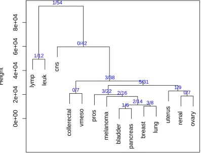
Figure 5 shows the test errors at each node of the complete linkage tree, for the 14 tumor data set.
3. Application to Other Cancer Microarray Data Sets
lymp
leuk
cns
collerectal
vmeso
pros
melanoma
bladder
pancreas
breast
lung
uterus
renal
ovary
0e+00
2e+04
4e+04
6e+04
8e+04
Height
1/6 2/14 3/8
2/16 0/7
3/22
0/7 1/9
5/31 3/38
1/12
0/42 1/54
Figure 5: Test errors for the 14 tumor data set using the complete linkage approach. Error rates at each decision junction is shown: notice that the errors tend to increase farther down the tree.
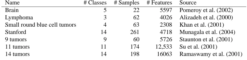
Name # Classes # Samples # Features Source
Brain 5 22 5597 Pomeroy et al. (2002)
Lymphoma 3 62 4026 Alizadeh et al. (2000)
Small round blue cell tumors 4 63 2308 Khan et al. (2001)
Stanford 14 261 4718 Munagala et al. (2004)
9 tumors 9 60 5726 Staunton et al. (2001)
11 tumors 11 174 12,533 Su et al. (2001)
14 tumors 14 198 16063 Ramaswamy et al. (2001)
Table 2: Summary of data sets for comparative study
.
Data set Nearest centroids SVM (OVO) MT(Single) MT(Complete) MT(Greedy) Brain 0.236(0.026) 0.207(0.022) 0.229(0.018) 0.229(0.021) 0.221(0.017) Lymphoma 0.010(0.006) 0.000(0.000) 0.000(0.000) 0.000(0.000) 0.000(0.000) SRBCT 0.065(0.020) 0.011(0.011) 0.014(0.014) 0.014(0.014) 0.014(0.014) Stanford 0.075(0.006) 0.063(0.006) 0.070(0.005) 0.079(0.007) 0.072(0.005) 9 tumors 0.478(0.009) 0.507(0.014) 0.526(0.013) 0.522(0.014) 0.545(0.014) 11 tumors 0.139(0.006) 0.110(0.005) 0.106(0.005) 0.106(0.005) 0.110(0.005) 14 tumors 0.493(0.007) 0.345(0.006) 0.318(0.007) 0.322(0.007) 0.315(0.007)
Table 3: Mean test error rates (standard errors) over 50 simulations, from various cancer microarray data sets. SVM (OVO) is the support vector machine, using the one-versus-one approach; each pairwise classifier uses a large value for the cost parameter, to yield the maximal margin classifier; MT are the margin tree methods, with different tree-building strategies.
4. Feature Selection
The classifiers at each junction of the margin tree each use all of the features (genes). For in-terpretability it would be clearly beneficial to reduce the set of genes to a smaller set, if one can improve, or at least not significantly worsen, its accuracy. How one does this depends on the goal.
The investigator probably wants to know which genes have the largest contribution in each classifier. For this purpose, we rank each gene by the absolute value of its coefficient ˆβj. Then to
form a reduced classifier, we simply set to zero the first nkcoefficients at split k in the margin tree.
We call this “hard-thresholding”.
How do we choose nk? It is not all clear that nk should be the same for each tree split. For
example we might be able to use fewer genes near the top of the tree, where the margins between the classes is largest.
Our strategy is as follows. We compute reduced classifiers at each tree split, for a range of values of nk, and for each, the proportion of the full margin achieved by the classifier. Then we use
a common valueαfor the margin proportion throughout the tree. This strategy allows the classifiers at different parts of the tree to use different number of genes. In real applications, we use tenfold cross-validation to estimate the best value forα.
10 50 500 5000
20
25
30
35
mean number of genes
error
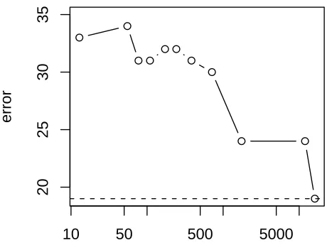
Figure 6: 14 tumor data set: Test errors for reduced numbers of genes.
the 13 tree junctions is shown along the horizontal axis. We see that average number of genes can be reduced from about 16,000 to about 2,000 without too much loss of accuracy. But beyond that, the test error increases.
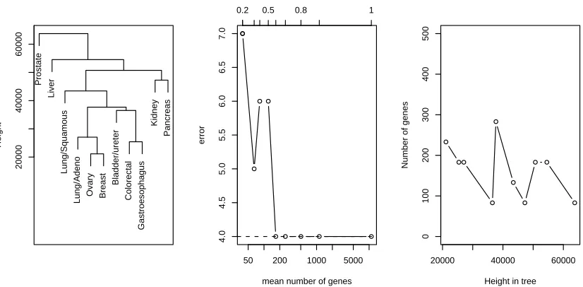
Figure 7 shows a more successful application of the feature selection procedure. The figure shows the result for one training/test split of the 11 class data (12,533 genes) described earlier. With no feature selection the margin tree (left panel) achieves 4/61 errors, the same as the one-versus one support vector machine. Hard-thresholding (middle panel) also yields 4 errors, with an average of just 167 genes per split. The margin proportion is shown at the top of the plot. The right panel shows the number of genes used as a function of the height of the split in the tree, for margin proportion 0.6.
The feature selection procedure described above is simple and computationally fast. Note that having identified a set of features to be removed, we simply set their coefficients ˆβi to zero. For
Prostate
Liver
Lung/Squamous
Lung/Adeno Ovary Breast
Bladder/ureter
Colorectal
Gastroesophagus
Kidney
Pancreas
20000
40000
60000
Height
50 200 1000 5000
4.0
4.5
5.0
5.5
6.0
6.5
7.0
mean number of genes
error
0.2 0.5 0.8 1
20000 40000 60000
0
100
200
300
400
500
Height in tree
Number of genes
Figure 7: Results for 11 tumor data set. The left panel shows the margin tree using complete link-age; the test errors from hard-thresholding are shown in the middle, with the margin proportionαindicated along the top of the plot; for the tree usingα=0.6, the right panel shows the resulting number of genes at each split in the tree, as a function of the height of that split.
4.1 Results on Real Data Sets
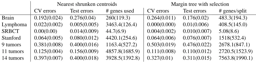
Table 4 shows the results of applying the margin tree classifier (complete linkage) with feature selection, on the data sets described earlier. Tenfold cross-validation was used to choose the margin fraction parameterα, and both CV error and test set error are reported in the table. Also shown are results for nearest shrunken centroids (Tibshirani et al., 2001), using cross-validation to choose the shrinkage parameter. This method starts with centroids for each class, and then shrinks them towards the overall centroid by soft-thresholding. We see that (a) hard thresholding generally improves upon the error rate of the full margin tree; (b) margin trees outperform nearest shrunken centroids on the whole, but not in every case. In some cases, the number of genes used has dropped substantially; to get smaller number of genes one could look more closely at the cross-validation curve, to check how quickly it was rising.
If two genes are correlated and both contribute too the classifier, they might both remain in the model, under the above scheme. One the other hand, if there is a set of many highly correlated genes that contribute, their coefficients will be diluted and they might all be removed.
0 2000 4000 6000 8000 10000 12000
0
10000
30000
Number of genes
Margins
Top split in tree
Simple Recomputed RFE
0 2000 4000 6000 8000 10000 12000
0
5000
15000
Number of genes
Margins
Bottom split in tree
Simple Recomputed RFE
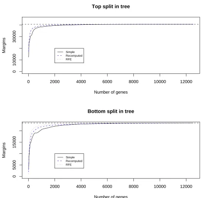
Figure 8: Results for the 11 tumor data set: margins achieved by the maximum margin classifier using simple hard thresholding without recomputing the weights (black points), with re-computation (blue points) and recursive feature elimination (red points). Top panel refers to the top split in the margin tree; bottom panel refers to the bottom split.
Nearest shrunken centroids Margin tree with selection CV errors Test errors # genes used CV errors Test errors # genes/split Brain 0.192(0.024) 0.276(0.04) 260(119.3) 0.264(0.011) 0.176(0.02) 483.3(194.3) Lymphoma 0.022(0.002) 0.005(0.005) 3463.4(126.4) 0.000(0.000) 0.01(0.006) 408.5(145.0) SRBCT 0.00(0.00) 0.014(0.009) 44.7(6.9) 0.004(0.002) 0.010(0.007) 5.08(8.6) Stanford 0.064(0.005) 0.080(0.012) 4420.1(254.6) 0.064(0.006) 0.076(0.007) 1518(532.4) 9 tumors 0.381(0.008) 0.400(0.016) 1163.4(527.2) 0.503(0.019) 0.476(0.022) 2678.1(847.1) 11 tumors 0.125(0.004) 0.156(0.009) 4857.8(1685.9) 0.111(0.008) 0.110(0.012) 2720.5(1523.9) 14 tumors 0.397(0.007) 0.400(0.018) 3928.5(1392.8) 0.327(0.01) 0.311(0.015) 7563.8(1990.1)
Table 4: CV and test error rates for nearest shrunken centroids and margin trees with feature se-lection by simple hard thresholding. The rightmost column reports the average number of genes used at each split in the tree.
5. Discussion
The margin-tree method proposed here seems well suited to high-dimensional problems with more than two classes. It has prediction accuracy competitive with multiclass support vector machines and nearest centroid methods, and provides a hierarchical grouping of the classes.
All of the classifiers considered here use a linear kernel, that is, they use the original input features. The construction of margin tree could also be done using other kernels, using the support vector machine framework. The greedy algorithm and linkage algorithms will work without change. However in the p>N case considered in this paper, a linear SVM can separate the data, so the utility of a non-linear kernel is not clear. And importantly, the ability to select features would be lost with a non-linear SVM.
We have restricted attention to the case p>N in which the classes are separable by a hyperplane. When p<N and the classes may not be separable, our approach can be modified to work in principle but may not perform well in practice. The nodes of the clustering tree will be impure, that is contain observations from more than one class. Hence a larger tree—one with more leaves than there are classes—might be needed to effectively classify the observations.
In addition to the papers on the multiclass support vector classifier mentioned earlier, there is other work related to our paper. The decision tree methods of Breiman et al. (1984) (“CART”) and Quinlan (1993) use top-down splitting to form a binary tree, but use other criteria (different from the margin) for splitting. With pN, splits on individual predictors can get unwieldy and exhibit high variance. The use of linear combination splits is closer to our approach, but again it is not designed for large numbers of predictors. It does not produce a partition of the classes but rather operates on individual observations.
Closely related to CART’s linear combination splits is the FACT approach of Loh and Vanichse-takul (1988) and the followup work of Kim and Loh (2001). These use Fisher’s linear discriminant function to make multi-way splits of each node of the tree. While linear discriminants might per-form similarly to the support vector classifier, the latter has the maximum margin property which we have exploited in this paper.
decision trees with support vector classifiers at the node, but do not discuss adaptive construction of the tree topology. Park and Hastie (2005) propose hierarchical classification methods using nearest centroid classifiers at each node. They use clustering methods to find the topology of the tree, and their paper has some ideas in common with this one. In fact, the mixture model used for each merged node gives a decision boundary that is similar to the support vector classifier. However the maximum margin classifier used here seems more natural and the overall performance of the margin tree is better.
Acknowledgments
We would like the thank the referees for helpful comments that led to improvements in this manuscript. Tibshirani was partially supported by National Science Foundation Grant DMS-9971405 and National Institutes of Health Contract N01-HV-28183. Trevor Hastie was partially supported by grant DMS-0505676 from the National Science Foundation, and grant 2R01 CA 72028-07 from the National Institutes of Health.
References
A. Alizadeh, M. Eisen, R. E. Davis, C. Ma, I. Lossos, A. Rosenwal, J. Boldrick, H. Sabet, T. Tran, X. Yu, Pwellm J., G. Marti, T. Moore, J. Hudsom, L. Lu, D. Lewis, R. Tibshirani, G. Sherlock, W. Chan, T. Greiner, D. Weisenburger, K. Armitage, R. Levy, W. Wilson, M. Greve, J. Byrd, D. Botstein, P. Brown, and L. Staudt. Identification of molecularly and clinically distinct sub-stypes of diffuse large b cell lymphoma by gene expression profiling. Nature, 403:503–511, 2000.
K. Bennett and J. Blue. A support vector machine approach to decision trees. Technical report, Rensselaer Polytechnic Institute, Troy, NY, 1997. R.P.I Math Report No. 97-100.
L. Breiman, J. Friedman, R. Olshen, and C. Stone. Classification and Regression Trees. Wadsworth, 1984.
I. Guyon, J. Weston, S. Barnhill, and V. Vapnik. Gene selection for cancer classification using support vector machines. Machine Learning, pages 389–422, 2002.
J. Khan, J. S. Wei, M. Ringn´er, L. H. Saal, M. Ladanyi, F. Westermann, F. Berthold, M. Schwab, C. R. Antonescu, C. Peterson, and P. S. Meltzer. Classification and diagnostic prediction of cancers using gene expression profiling and artificial neural networks. Nature Medicine, 7:673– 679, 2001.
H. Kim and W.Y. Loh. Classification trees with unbiased multiway splits. Journal of the American Statistical Association, 96:589–604, 2001.
Y. Lee, Y. Lin, and G. Wahba. Multicategory support vector machines, theory, and application to the classification of microarray data and satellite radiance data. Journal of the Amer. Statist. Assoc., 99:67–81, 2004.
K. Munagala, R. Tibshirani, and P. Brown. Cancer characterization and feature set extraction by discriminative margin clustering. BMC Bioinformatics, 5:5–21, 2004.
M. Y. Park and T. Hastie. Hierarchical classification using shrunken centroids. Technical report, Stanford University, 2005.
S. L. Pomeroy, P Tamayo, M. Gaasenbeek, L. M. Sturla, M. Angelo, M. E. McLaughlin, J. Y. Kim, L. C. Goumnerova, P. M. Black, C. Lau, J. C. Allen, D. Zagzag, J. M. Olson, T. Curran, C. Wet-more, J. A. Biegel, T. Poggio, S. Mukherjee, R. Rifkin, A. Califano, G. Stolovitzky, D. N. Louis, J. P. Mesirov, E. S. Lander, and T. R. Golub. Prediction of central nervous system embryonal tumour outcome based on gene expression. Nature, 5:436–42, 2002.
R. Quinlan. C4.5: Programs for Machine Learning. Morgan Kaufmann, San Mateo, 1993.
S. Ramaswamy, P. Tamayo, R. Rifkin, S. Mukherjee, C. Yeang, M. Angelo, C. Ladd, M. Reich, E. Latulippe, J. Mesirov, T. Poggio, W. Gerald, M. Loda, E. Lander, and T. Golub. Multiclass cancer diagnosis using tumor gene expression signature. PNAS, 98:15149–15154, 2001.
S. Rosset, J. Zhu, and T. Hastie. Margin maximizing loss functions. In Advances in Neural Infor-mation Processing Systems, (NIPS*2005), 2005.
A. Statnikov, C.F. Aliferis, I. Tsamardinos, D. Hardin, and S. Levy. A comprehensive evaluation of multicategory classification methods for microarray gene expression cancer diagnosis. Bioinfor-matics, pages 631–43, 2004.
J.E. Staunton, D.K. Slonim, H.A. Coller, P. Tamayo, M.J. Angelo, U. Park, J. Scherf, J.K. Lee, W.O. Reinhold, and J.N. Weinstein. Chemosensitivity prediction by transcriptional profiling. Proc. Natl Acad. Sci. USA, 98:10787–10792, 2001.
A.I. Su, J.B. Welsh, L.M. Sapinoso, S.G. Kern, P. Dimitrov, H. Lapp, P.G. Schultz, S.M. Pow-ell, C.A. Moskaluk, H.F. Frierson, Jr, and G.M. Hampton. Molecular classification of human carcinomas by use of gene expression signatures. Cancer Research, 61:7388–7393, 2001.
R. Tibshirani. The lasso method for variable selection in the cox model. Statistics in Medicine, 16: 385–395, 1997.
R. Tibshirani, T. Hastie, B. Narasimhan, and G Chu. Diagnosis of multiple cancer types by shrunken centroids of gene expression. Proc. Natl. Acad. Sci., 99:6567–6572, 2001.
V. Vural and J. G. Dy. A hierarchical method for multi-class support vector machines. 2004. International Conference on Machine Learning; Proceeding Series; Vol. 69.
J. Weston and C. Watkins. Multi-class support vector machines. In M. Verleysen, editor, Proceed-ings of ESANN99. D. Facto Press, Brussels, 1999.