Pintar2013-RegionalHomogenization

Regional homogenization of surface temperature records using robust

statistical methods

A. L. Pintar, A. Possolo, and N. F. Zhang

Citation: AIP Conf. Proc. 1552, 1054 (2013); doi: 10.1063/1.4819689

View online: http://dx.doi.org/10.1063/1.4819689

View Table of Contents: http://proceedings.aip.org/dbt/dbt.jsp?KEY=APCPCS&Volume=1552&Issue=1

Published by the AIP Publishing LLC.

Additional information on AIP Conf. Proc.

Journal Homepage: http://proceedings.aip.org/

Journal Information: http://proceedings.aip.org/about/about_the_proceedings

Top downloads: http://proceedings.aip.org/dbt/most_downloaded.jsp?KEY=APCPCS

Regional Homogenization of Surface Temperature Records

Using Robust Statistical Methods

A. L. Pintar, A. Possolo, and N. F. Zhang

Statistical Engineering Division Information Technology Laboratory National Institute of Standards and Technology

100 Bureau Drive Mail Stop 8980 Gaithersburg, MD 20899

Abstract. An algorithm is described that is intended to estimate and remove spurious influences from the surface temperature record at a meteorological station, which may be due to changes in the location of the station or in its environment, or in the method used to make measurements, and which are unrelated to climate change, similarly to [1]. The estimate of these influences is based on a comparison of non-parametric decompositions of the target series with series measured at other stations in a neighborhood of the target series. The uncertainty of the estimated spurious artifacts is determined using a statistical bootstrap method that accounts for temporal correlation structure beyond what is expected from seasonal effects. Our computer-intensive bootstrap procedure lends itself readily to parallelization, which makes the algorithm practicable for large collections of stations. The role that the proposed procedure may play in practice is contingent on the results of large-scale testing, still under way, using historical data.

Keywords: Autocorrelation, Change-Point, LOESS, Homogenization, Temperature Series.

INTRODUCTION

Surface temperature records from meteorological stations may be corrupted by spurious artifacts. These corruptions can arise from changes in the location of the station or in its environment, e.g. moving a station from the roof of a building to an open field. They also may be caused by changing the method used to make measurements, e.g. changing from liquid in glass to digital. These influences are unrelated to climate change, but they can severely impact an estimate of long term trend. Our basic goal of removing the impact that these spurious influences have on estimates of long term trend is similar to what the authors of [1] consider.

The procedure for removing spurious artifacts that is suggested and illustrated here, is based on a non-parametric decomposition of surface temperature records into trend, seasonal, and remainder components, at a target station and at each of its neighboring stations. Using these decompositions, we calculate the homogenization correction that will be applied to the target series. The statistical significance of the correction is assessed using the non-parametric bootstrap in a way that recognizes that surface temperature records typically exhibit autocorrelations beyond those that are induced by seasonal effects.

This algorithm is intended for application to records that exhibit change-points whose presence has been previously detected, and whose statistical significance has been ascertained, using methods described in [2], for example. The portion of the algorithm that serves to assess the uncertainty and gauge the statistical significance of the homogenization correction is compute-intensive. However, both calculating the correction, and assessing its uncertainty, lend themselves readily to parallelization, so that, should n(or, ideally, n2) processors be available, where ndenotes the number of neighbors of the target station, the algorithm becomes practicable for large collections of stations. The algorithm is currently implemented in the R environment for statistical modeling, computing, and graphics [3], which is freely available as open source and executables for most computing platforms.

ALGORITHM

accommodate daily measurements. Next, define start and end dates (each specified as a month and year combination) for the change-point detection and adjustment of the target station series, so that a reasonably large number of stations in

N

have temperature measurements between these dates. Use those start and end dates to define a time series y_T for the target station, and time series

{x_j:j 1,..., }n for the neighboring stations, all consisting of monthly averages (or maxima, or minima), and all possibly including missing values. Next, missing values are imputed. For each of the twelve months of the year k 1,...,12, let wkdenote the median of all temperature measurements, made at the target and at neighboring stations, across all years in a “reference” period, which may be the whole record between the start and end dates or only a subset of it. Replace each missing value in each station’s time series by the median computed in the previous step for the month that the missing value corresponds to. The best, general purpose imputation method still needs to be determined. Obviously, imputation is particularly challenging when there are long blocks of consecutive missing observations: it may be unrealistic to impute long blocks of consecutive missing observations and even to use stations in this homogenization procedure with such blocks. One reviewer has pointed out that if the station temperature series should have multi-decadal variations, this simple imputation method may “scramble” the signal expressed in these variations, especially if there are long blocks of missing values. In the series used to illustrate the proposed homogenization procedure this is not the case.

Now, we have n+1 time series of the same length with no missing values, and we decompose each of them as

( ) ( ) ( )

z m z s z r z , (1)

wherem z( ) is the seasonal component, s z( )is the trend component, and r z( )is the remainder of the time series z. This can be accomplished using the R function stl [4], with typical output illustrated in Fig 1.

The trend component of the target series s y( T)

can be interpreted as the climate signal that we are attempting to homogenize, which we will do using the trend component of the series at neighboring stations. We develop our procedure under the assumption that all neighboring stations are free of spurious influences. This is not necessarily the case in practice, but our procedure should be robust to neighboring stations containing spurious influences because the final correction combines information

from all neighboring stations in a robust way (medians are used). In fact, even if all neighboring

FIGURE 1. Reno - Seasonal DecompositionThe top panel (whose vertical axis is labeled “data”) depicts the

monthly minima at the Reno, NV, station, and the lower

panels depict the estimated seasonal component

m

ˆ

(

y

_T

)

, the estimated trend component

s

ˆ

(

y

_T

)

, and the estimated

remainder

r

ˆ

(

y

_T

)

, as produced by R function stl. The gray bars on the right hand side of the plots represent the same range of temperatures in all the panels, thus facilitating comparing the amplitudes of the oscillations exhibited by the different components.

stations suffer from spurious influences this procedure may still perform as intended. The conditions under which this is the case are reported shortly. One reviewer has pointed out that in regions whose surface temperature records are centrally managed, it is possible that the records at the majority of neighboring stations may suffer from similar, synchronous spurious influences: in such circumstances, it is unlikely that any homogenization procedure based on local inter-comparisons will be satisfactory.

To homogenize s y( T)we assume the following

models for the trend component of the target and neighboring series: s yt( T) bT V Ht t, and

( ) ; 1, 2,...,

t j j t

s x b V j n, where the t subscripts

series. In other words, we assume that if the target series were free of spurious influences, its trend would simply be a shifted version of the trend of the neighboring stations. Let s y( T)and s x( j)be the average over all epochs of the trend component of the target series and of its jth neighbor. Then,

( )_{t T}

s y b

V H

, (s xj) bj V, and

[ (t T) ( T)] [ (t j) ( j)]

t

s y s y s x s x

H

H

,

(2)

which is a shifted version of Ht. As a result, if (2) is subtracted from s y_t( _T)we get a true climate signal that is free of Ht but is shifted by H . Since H is unknown, all that this homogenization procedure can possibly achieve is to correct the trend of the record at the target station.

Under the assumed model, if the trend components were known without error, (2) would be the same for each of the neighboring stations. However, since the trend components are estimated from data this is not the case. To combine the information from all of the neighboring stations we do the following. First, (2) is computed for each of the n neighboring stations. Next, the median of those values (at each epoch t) is computed over all neighboring stations. We refer to this time series of medians as HtmedHmed. Last, we smooth

med med t

H H using for example a re-descending M estimator [5] as implemented in the R function loess [6] for protection against outliers, and that smoothed curve is our estimate of H H_t , which can then be subtracted from the estimated trend of the target series.

Now, supposing that neighboring stations are not free of spurious influences, let

H

_tj represent a spurious influence at time

t

of neighboring station

j

and

H

jbe the average of

H

_tj over

t

. Then, (2) is

no longer

H

_t

H

but instead

H

_t

H

H

j

H

_tj. However, since we calculate (2) for each neighboring station and then take the median, as long as the median of

H

j

H

_tj over

j

(the neighboring stations) is zero, the algorithm will perform as stated. When this is not the case, an examination of the corrected trend may reveal it, i.e. spurious influences that were visible originally may still be visible in the corrected trend.

ASSESSING UNCERTAINTY

In the previous section, we noted that the trend component for the time series at each station is estimated from data. Since the estimate of H Ht is constructed from those estimates, its uncertainty should be quantified, which we do by employing the non-parametric bootstrap [7].

Let ete denote the estimate of H t H. The residuals for each station after decomposition by stl are denoted by r y( T), r x( )1 , …, and r x( n). We assume that any of the remainders, or local fluctuations, that are neither seasonal nor reflect trend could conceivably have been observed at the target or neighboring stations. The bootstrap procedure is a repetition of the following steps n_B times.

1. Sample with replacement n+1 of the residual time series, and denote them r*(y_T), r x*( )1 ,

, and *_{( )}

n

r x .

2. Form *

T

y and * 1

x through *

n

x , the bootstrap sample as y*_T m(y_T)s(y_T)r*(y_T) and

* *

( ) ( ) ( )

j j j j x m x s x r x .

3. Carry out the homogenization procedure, to get * *

t

e e .

The nB time series,

* *

t

e e , represent the

uncertainty in time series e_te , which can be summarized as a time series of point-wise confidence bounds. It should be noted that this evaluation does not capture contributions from sources of uncertainty that affect all the records in the same way (systematic errors).

SIMULATION RESULTS

To assess the adequacy of this procedure, data records were simulated according to (1) for a target station and for 50 neighboring stations. The seasonal component was m_t 12 2[(t 1) (mod12)], where the subscript t=1,2, …, 600 refers to the epochs of the time series, here representing 50 years. The trend component was s_t 0.01t, which describes a climatic signal inducing a monthly increase of 0.01°C in average surface temperature. For the target series, a change point of -5°C was introduced at time t = 301. Note that the same seasonal and trend components are used for the target station and for all of the neighboring stations. The remainder, j

t

r , is

the sum of two random components: j j t t t

r AI ,

either the target station or one of the neighboring stations. The first component of the remainder,At, is a stationary autoregressive process of order 1 (AR(1)) with mean zero and dependence parameter 0.5, and innovations from a Student’s t-distribution with 3 degrees of freedom. The second component of the remainder, j

t

I , comprises independent Gaussian random variables with mean zero and variance two.

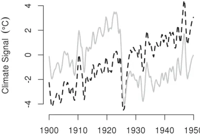
Fig. 2 shows the results of applying the homogenization procedure to the simulated data: the solid curve is the estimate of the original trend for the target series, and the dashed curve is the homogenized trend. In the original estimate of the trend (solid curve) we clearly see the change-point at

t=301, or January 1926; however, by applying the homogenization algorithm the change-point has been removed and, the climate signal has been preserved.

FIGURE 2. Results of the homogenization algorithm applied to the simulated data. The solid curve is the original estimate of trend from the target series. The dashed curve is the trend after applying the homogenization algorithm.

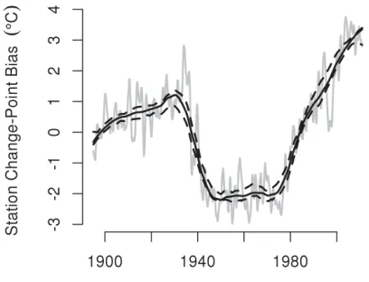
Fig. 3 depicts an estimate of med med t

H H (solid grey curve), ete (solid black curve), and an upper and lower point-wise bound for H H_t (dashed curves). The uncertainty in ete is very small for some epochs as the dashed curves blend into the solid black curve.

Fig. 3 also suggests that the loess procedure slightly over smoothes the change-point, which induces the larger than expected dip in the homogenized trend at the beginning of 1926 (dashed curve) in Fig 2. There are at least two different ways to remedy this over smoothing. First, we could simply change the bandwidth parameter in the loess procedure. Here however, this is undesirable

FIGURE 3. For the simulated data, H_tmedHmed (solid grey cuve), e_te (solid black cuve), and upper and lower point-wise bounds for H H_t (dashed curves).

because it leads to too little smoothing at epochs away from the change-point.

Another option is to change the smoothing procedure from loess to adaptive weights smoothing (AWS) [8]. The propagation-separation approach to AWS [9] is implemented in the function aws defined in the R package of the same name [10]. The AWS procedure was developed to detect discontinuities in images, but it is useful for time series too, and it may not over smooth change points because they are a type of discontinuity. Figs. 4 and 5 depict the correction and the trend after applying this correction, computed using the aws smoother instead of loess. Fig. 4 shows that the dip in the homogenized trend around 1926 is much smaller than in Fig. 2. Further, the slope of the vertical shift representing the change point in 1926 is more extreme in Fig. 5 than in Fig. 3. Thus, the aws procedure is performing as expected, and not smoothing out the change point as much as loess.

RENO RESULTS

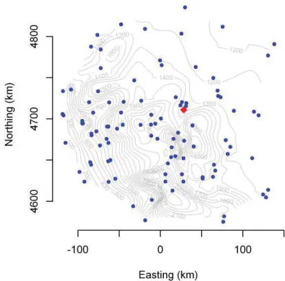
Our homogenization algorithm was also applied to data from stations near Reno, NV. The target station is at Reno Tahoe International Airport, and it has Cooperative Station identifier 266779 and World Meteorological Organization identification number 72488. The 98 neighboring stations are within 150 km of the Reno station. Fig. 6 shows the locations of the target and neighboring stations.

FIGURE 4. Results of the homogenization algorithm applied to the simulated data using aws instead of loess. The solid curve is the original estimate of trend from the target series. The dashed curve is the corrected trend.

FIGURE 5. For the simulated data, an estimate of med med

t

H H (solid grey cuve), e_te (solid black cuve), and upper and lower point-wise bounds for H H_t (dashed curves) using aws instead of loess.

( T)

s y , and the dashed curve depicts the estimated

( T)

s y after homogenization. Note that after homogenization, the estimated trend is mostly horizontal, neither increasing nor decreasing. One reviewer has pointed out that the homogenization procedure may have been too aggressive in this case because the result does not show the trend in surface temperatures documented for the period of interest in the western United States [13]. This suggests the possible need for more carefully tuning the parameters that determine the procedure, e.g. the bandwidth parameter in the loess procedure, taking into account all the information available for the region where it will be applied.

FIGURE 6. Neighborhood of the target station at Reno, NN, which comprises 98 other stations within about 150 km of the target station. The easting and northing coordinates were computed using facilities from the R package rgdal [11], by transforming the longitude and latitude according to a Lambert conformal conical projection whose reference longitude was the target

station’s, and whose reference parallels just bounded the

latitudes of all neighboring stations.

FIGURE 7. Results of applying our homogenization algorithm to the Reno data. The solid curve is the original estimate of trend from the target series. The dashed black curve is the result of applying the homogenization algorithm to the solid grey curve using the 98 neighboring stations.

around 1996-1998, corresponding to the station’s temporary relocation to the south end of the runway.

FIGURE 8. For the Reno data, H_tmedHmed (solid grey curve), e_te (solid black curve), and an upper an lower point-wise bound for H H_t (dashed curves).

CONCLUSION

We have described an algorithm for homogenizing the trend of a time series of temperature measurements at a target station. The algorithm works by comparing the target stations to neighboring stations whose trends are assumed to be homogeneous. However, even if the neighboring stations are not all homogeneous, we expect that our procedure still will produce reasonable results owing to built-in robustness, provided such influences do not affect a majority of neighboring stations synchronously. The algorithm is based on a set of statistical tools that are implemented in the free, open source, R language for statistical computing.

We demonstrated the algorithm on a set of simulated data where the trend of the target station contained an abrupt change point. The algorithm correctly removed the abrupt change, while preserving the true trend that was present in the time series. The algorithm was also applied to real data from Reno, NV. In this case the algorithm removed an abrupt change in the middle of the series of temperatures as well as a positive trend towards the end of the series.

A bootstrap procedure to assess the uncertainty in

t

e e , our estimate of the spurious influences on the target series was also described. While the procedure is computationally expensive, it is very useful, because it allows us to decide whether homogenization adjustments are warranted. For instance, if we assess the uncertainty in ete, and

the possibility that H Ht is constantly zero seems plausible, we might conclude that the target series is free of spurious influences. In such cases, we would prefer the original series to the homogenized series. This was not the case in either the simulated data or the Reno data where spurious influences were quite obviously present.

REFERENCES

1. Menne, M. J., and Williams, C. N. Jr., Journal of

Climate22, 1700-1717 (2009).

2. Possolo, A., Pintar, A. L., and Zhang N. F., “Statistical Methods for Change-Point Detection in Surface Temperature Records”, in Temperature: Its Measurement and Control in Science and Industry,

Vol. 8, edited by C.W. Meyer, Melville, NY: American

Institute of Physics, 2013.

3. R Development Core Team, R: A Language and

Environment for Statistical Computing, Vienna: R

Foundation for Statistical Computing, 1020, URL

http://CRAN.R-project.org ISBN 3-900051070. 4. Cleveland, R. B., Cleveland, W. S., McRae, J. E., and

Terpenning, I., Journal of Official Statistics, 6, 3-73 (1999).

5. Huber, P. J., and Ronchetti, E. M., Robust Statistics, Hoboken: John Wiley & Sons, 2009.

6. Cleveland, W. W., and Devlin, S., J., Journal of the

American Statistical Association83, 596-610 (1988).

7. Efron, B., and Tibshirani, R. J., An Introduction to the

Bootstrap, New York: Chapman & Hall, 1993.

8. Polzehl, J., and Spokoiny, V., Journal of the Royal

Statistical Society, 62, 335-354 (2000).

9. Polzehl, J., and Spokoiny, V., Probability Theory and

Related Fields, 135, 335-362 (2006).

10. Polzehl, J., aws: Adaptive Weights Smoothing, 2010 URL http://CRAN.R-project.org/package=aws R package version 1.6-2.

11. Keitt, T. H., Bivand, R., Pebesma, E., and Rowlingson,

B., rgdal: Bindings for the Geospatial Data

Abstraction Library, 2010,URL

http://CRAN.R-project.org/package=rgdal R package version 0.6-33. 12. Menne, M., Easterling, D., Vose, R., and Williams, C.

(2009) Areas of potential collaboration in the use of statistical approaches for providing in situ climate records. Briefing to the Statistical and Applied Mathematical Sciences Institute (SAMSI), Research Triangle Park, North Carolina —September 17, 2009. 13. Udall, B., and Bates, G. (2007) Climatic and

Hydrologic Trends in the Western U.S.: A Review of Recent Peer-Reviewed Research. Intermountain West

Climate Summary, January 2007. Western Water

Assessment, and joint project of University of Colorado and NOAA/ESRL Physical Sciences Division.