Journal of Hydraulic Structures
J. Hydraul. Struct., 2018; 4(2):1-9 DOI: 10.22055/JHS.2018.26273.1080
A Mass Conservative Method for Numerical Modeling of
Axisymmetric flow
Roza Asadi1
Abstract
In this paper, the axisymmetric flow toward a pumping well has been numerically solved by the cell-centered finite volume method. The numerical model is discretised over unstructured and triangular-shaped grid which allows simulating inhomogeneous and complex-shaped domains. Due to the non-orthogonality of the irregular grids, the multipoint flux approximation (MPFA) schemes are used to discretize the flux term. In this work, the diamond scheme as the MPFA method has been employed and the least square method is applied to express the full discrete form of the vertex-values of the hydraulic head. The scheme has been verified via the Theis solution, as a milestone in well hydraulics. The numerical results show the capability of the developed model in evaluating transient drawdown in the confined aquifers. The proposed numerical model leads to the stable and local conservative solutions contrary to the standard finite element methods. Also this numerical technique has the second order of accuracy.
Keywords: Axisymmetric radial flow, Cell-centered finite volume method, MPFA method, Diamond scheme.
Received: 11 March 2018; Accepted: 29 Jun 2018
1. Introduction
Groundwater accounts for about 30 percent of the world's supply of fresh water. In arid and semi-arid regions this resource serves as an alternative to the surface reservoirs of water. These issues make well hydraulics an important aspect in hydrological and water science problems. The mathematical analysis of well pumping on head decline in confined aquifers first provided by Theis in 1935 [1]. The analytical solutions for other types of aquifers such as leaky and unconfined aquifer were obtained by Hantush and Jacoub [2] and Neuman [3-6], respectively. However, the analytical solutions are limited to the ideal cases. Thus, numerical methods have been developed to model the real and complicated circumstances. Despite the traditional numerical schemes such as the standard finite element method developed extensively to model the groundwater problems, it suffers from the numerical oscillations especially in inhomogeneous porous media [7-10]. In order to resolve the numerical instabilities and provide
1 Department of Civil Engineering, K.N. Toosi University of Technology, Tehran, Iran, [email protected]
mass conservative solution, the finite volume methods (FVMs) have been formulated to simulate the groundwater flow equation [10-15]. Since the unstructured grid is the most efficient and flexible mesh to model the complex geometries and sharp heterogeneities [16], this type of mesh is applied in this study. Due to non-orthogonality of the irregular grids, MPFA schemes are used to discretize the flux term [17,18]. In this work, the diamond scheme as the MPFA method has been employed on the unstructured triangular grids [19-23]. Moreover, the least square method is applied to express the full discrete form of the vertex-values of the hydraulic head. This procedure results in the cell-centered finite volume method (CC-FVM). It was demonstrated in [15, 21] that this scheme provides second-order accurate solutions.
In [13], this discretization scheme was combined with the mechanics equation to simulate the Biot's model [24] in two-dimensional domain. It was illustrated that the proposed numerical method result in stable and local conservative solutions. In addition, it was shown that the unstructured grid makes the model well-suited for simulating heterogeneous domains and complicated geometries [13].
The axisymmetric flow toward a pumping well has been numerically solved by the cell-centered finite volume method. Since the computational cost of the axially symmetric model is less than the equivalent three dimensional one, this simplification has been assumed in the formulations. Indeed, in this study the effectiveness of the model in simulating flow in confined aquifer subjected to pumping has been investigated.
2. Mathematical formulation
The governing equation for fluid flow in a confined aquifer is:
𝑆𝑠𝜕ℎ
𝜕𝑡+ div𝐯 = 𝑓 (1)
where 𝑆𝑠 is the specific storage coefficient which can be defined as 𝜌𝑤𝑔(𝛼 + 𝑛𝛽), 𝐯 = 𝐊̅∇ℎ is the Darcy's velocity, ℎ denotes the hydraulic head and 𝐊̅ is the tensor form of the hydraulic conductivity. t is time, 𝜌𝑤 denotes the density of fluid, 𝑛 is the porosity and 𝛼 and 𝛽 are the compressibility of aquifer and fluid, respectively. Finally, 𝑓 is a sink /source term.
The required boundary conditions can be written as follows:
ℎ = ℎ𝐷 on 𝛤ℎ (2)
𝐯. 𝐧 = 𝑞 on 𝛤𝑞 (3)
where ℎ𝐷 and 𝑞 are the boundary values of the hydraulic head and flux, respectively. The unit normal vector 𝐧is pointing outward from the boundaries which are defined as:
𝛤ℎ∪ 𝛤𝑞 = 𝜕Ω (4)
𝛤ℎ∩ 𝛤𝑞 = ∅ (5)
3. Numerical model
A detailed description of the numerical formulations is presented in this section. For this purpose at the first stage, the FVM method has been applied for discretizing the flow equation and then a diamond scheme has been implemented to approximate the flux term. As mentioned earlier the variation of the hydraulic properties in the angular direction has been neglected and the model simulates the planar domain.
3.1.1 The CC-FVM
∫ (𝑆𝑠𝜕ℎ
𝜕𝑡 + div𝐯) 𝑑V
Vi
= ∫ 𝑓𝑑V
V𝑖
(6)
where in the above equation 𝑑V is the volume element which is defined as 𝑟𝑑𝑟𝑑𝜃𝑑𝑧 in the cylindrical coordinates. For the axisymmetric case the above equation can be reduced to the double integral as follows:
∫ 𝑟 (𝑆𝑠𝜕ℎ
𝜕𝑡+ div𝐯) 𝑑Ω
Ωi
= ∫ 𝑟𝑓𝑑Ω
Ω𝑖
(7)
where 𝑑Ω is the area element such that 𝑑Ω = 𝑑𝑟𝑑𝑧, Ωi denotes the two dimensional control volume and 𝑟 and z are the radial and axial coordinates, respectively. By implementing theorem of Gauss–Green to Eq. (7), the integral form of the flow equation will read as:
∫ 𝑟 (𝑆𝑠𝜕ℎ 𝜕𝑡) 𝑑Ω
Ωi
− ∫ 𝐧. 𝐊̅∇ℎ
𝜕Ωi
𝑟𝑑Γ = ∫ 𝑟𝑓𝑑Ω
Ωi
(8)
The symbols 𝜕Ωi denotes the control volume's boundary. With approximating hydraulic head and the source/sink term at the centroid of the control volumes, the discretized form of the flow equation is obtained as follows:
𝑟̅𝑆𝑠𝜕ℎ𝑖
𝜕𝑡 |Ωi| + ∑ 𝑟𝑒𝑉𝑖𝑗|Γ𝑖𝑗|
Γ𝑖𝑗𝜖𝜕Ωi
= 𝑟̅𝑓𝑖|Ωi| (9)
in which ℎ𝑖 is cell-averaged value of the hydraulic head. Γ𝑖𝑗 is the internal edge between two adjoining cells (Ωi and Ωj) and the absolute value of Γ𝑖𝑗 (|Γ𝑖𝑗|) represents its length. 𝑉𝑖𝑗 denotes the flux across this edge and |Ωi| is used to present area of the control volume. 𝑟̅ and 𝑟𝑒 denote the radial distances from the cell center and the midpoint of the edge Γ𝑖𝑗. 𝑓𝑖 indicates the cell average of the sink/source term.
The velocity term is discretized with the equation proposed by Coudière et al. [20]:
𝑉𝑖𝑗= −
1 |Γ𝑖𝑗|
∫ 𝐧. 𝐊̅∇ℎ
Γ𝑖𝑗
𝑑Γ (10)
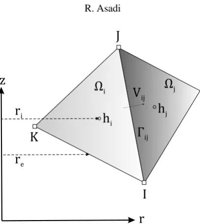
Figure 1. Symbols used in the numerical formulations
3.1.2 Approximating flux integral
As mentioned earlier, a diamond scheme as a multipoint flux approximation is applied to evaluate the flux at the interface of the cells. In this procedure, the gradient of hydraulic head is calculated with the values of head at the vertices and center of the cells [18-20, 22, 25]. Indeed, using only cell center values of hydraulic head result in inaccurate solution for the unstructured grids [18, 25]. The gradient of hydraulic head across the boundary Γ𝑖𝑗 is given by [13, 15, 19, 20, 23]:
𝝍𝑖𝑗 = (ℎ𝑗− ℎ𝑖
𝐷𝑖𝑗 − cot 𝜃
ℎ𝐽− ℎ𝐼 |Γ𝑖𝑗| ) 𝐧ij+
ℎ𝐽− ℎ𝐼
|Γ𝑖𝑗| 𝐭ij (11)
In the above equation, 𝐧ij indicates the unit normal of Γ𝑖𝑗 and is assumed that pointing from i to j (Fig. 2), and 𝐭ij is the tangent vectors of the respective face. As illustrated in figure 2, ℎ𝑖 and ℎ𝐼 are the head values at the centroid of cell 𝑖 and vertex 𝐼, and ℎ𝑗 and ℎ𝐽 are the corresponding values at the center of the control volume 𝑗 and node 𝐽, respectively. As shown in Fig.2, the parameter 𝐷𝑖𝑗 is defined as 𝐷𝑖𝑗= 𝑑𝑖𝑗+ 𝑑𝑗𝑖, in which 𝑑𝑖𝑗 and 𝑑𝑗𝑖 are the length of the lines between points 𝑖 and 𝑗 and the cell face, respectively [13, 15, 19, 20, 23]. Other parameters in Eq.(11) are illustrated in Fig.(2).
Figure 2. Parameters used in the multipoint flux stencil
h
iJ
I
K
Ω
iΓ
ijV
ijh
jΩ
jr
ir
er
z
i
j
I
d
ijd
ji
θ
n
ijt
ijCombining Eq. (10) and (11), yields the full discrete form of flux as [13, 19, 20]:
𝑉𝑖𝑗 = −𝜿𝝍𝑖𝑗. 𝐧ij (12)
In the above equation, the conductivity tensor 𝜿 is the full matrix which can be expressed as follows [13, 19, 20]:
𝜿 = 1
|Γ𝑖𝑗|∫ 𝐊Γ𝑖𝑗̅
𝑑Γ = [𝜅𝜅𝑛𝑛 𝜅𝑛𝑡
𝑡𝑛 𝜅𝑡𝑡] in (𝐧ij, 𝐭ij) (13)
By substituting Eqs. (10) and (12) into Eq. (11), the numerical flux reads as [13, 19, 20, 23]:
𝑉𝑖𝑗= −𝜅𝑛𝑛ℎ𝑗− ℎ𝑖
𝐷𝑖𝑗 − (𝜅𝑛𝑡− cot 𝜃𝜅𝑛𝑛)
ℎ𝐽− ℎ𝐼
|Γ𝑖𝑗| (14)
Finally by interpolating head values at vertices in terms of the cell center values, the FV discretization will be completed [18, 20]. Averaging procedure for computing the weight factors is the least squares algorithm [15, 19-22]. By applying this averaging procedure, ℎ𝐼 is calculated as follows:
ℎ𝐼= ∑ 𝑤𝑖ℎ𝑖 𝑁𝐼
𝑖=1
(15)
The above summation is done over the cells common to the point I, and the weighting function
𝑤𝑖 is defined for any control volume sharing vertex 𝐼 as [13, 19, 20]:
𝑤𝑖 =1 + 𝛬𝑟(𝑟𝑖− 𝑟𝐼) + 𝛬𝑧(𝑧𝑖− 𝑧𝐼)
𝑁𝐼+ 𝛬𝑟𝑅𝑟+ 𝛬𝑧𝑅𝑧 (16)
where 𝑟𝑖 and 𝑟𝐼 are the radial distances of the cell center 𝑖 and vertex 𝐼, respectively. 𝑧𝑖 and 𝑧𝐼 denote the vertical distances of 𝑖 and 𝐼 from the z-axis. Also the following equations are used to formulate other functions in Eq. (16) [13, 19, 20]:
𝛬𝑟 =
𝐼𝑟𝑧𝑅𝑧− 𝐼𝑧𝑧𝑅𝑟
𝐼𝑟𝑟𝐼𝑧𝑧− 𝐼𝑟𝑧2 (17)
𝛬𝑧 =
𝐼𝑟𝑧𝑅𝑟− 𝐼𝑟𝑟𝑅𝑧
𝐼𝑟𝑟𝐼𝑧𝑧− 𝐼𝑟𝑧2 (18)
𝐼𝑟𝑟= ∑(𝑟𝑖− 𝑟𝐼)2 𝑁𝐼
𝑖=1
(19)
𝐼𝑧𝑧= ∑(𝑧𝑖− 𝑧𝐼)2 𝑁𝐼
𝑖=1
(20)
𝐼𝑟𝑧= ∑(𝑟𝑖− 𝑟𝐼)
𝑁𝐼
𝑖=1
(𝑧𝑖− 𝑧𝐼) (21)
𝑅𝑟 = ∑(𝑟𝑖− 𝑟𝐼)
𝑁𝐼
𝑖=1
(22)
𝑅𝑧 = ∑(𝑧𝑖− 𝑧𝐼)
𝑁𝐼
𝑖=1
By substituting Eqs. (15) and (16) into Eq.(14), the final discrete form of this equation can be obtained. The similar procedure has been performed for all faces of each control volume to complete discretization of Eq.(9).
4 Numerical result
To verify the proposed scheme, the Theis solution has been solved and the numerical results have been compared with the analytical solutions. The validation demonstrates the effectiveness of the numerical technique for modeling the radial flow toward wells in confined aquifers. Moreover, to construct the triangular grids, NETGEN algorithm has been implemented as the mesh generator tool [26] and all of the numerical codes have been written in MATLAB 2010 software.
The first analytical solution for the drawdown problem in the confined aquifer was derived by Theis (1935) [1]. To simplify the problem the following assumptions have been made in the Theis solution:
1. The confined aquifer is considered as a homogeneous, isotropic porous media and has infinite horizontal extent.
2. The piezometric surface is considered horizontal prior to pumping.
3. The well is fully penetrated and the pumping rate is constant.
4. The radial flow towards well is horizontal.
5. The radius of the pumping well is very small.
6. The layer has uniform extent and confined top and bottom.
7. Water is released from the porous media as head declines [27, 28].
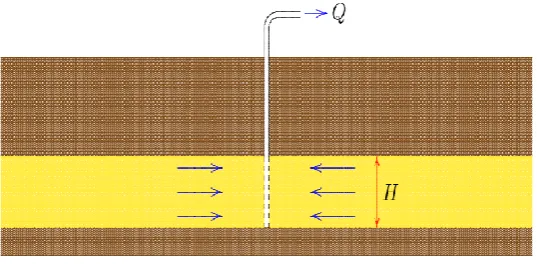
These conditions are illustrated in Fig. 3. With the above assumptions, the drawdown 𝑠′ is calculated as [27, 28]:
𝑠′= 𝑄
4𝜋𝑇∫
𝑒−𝑦
𝑦
∞
𝑢
𝑑𝑦 (24)
where𝑄 is the pumping rate, 𝑇 denotes transmissivity, the parameter 𝑢 is defined as 𝑟 2𝑆
4𝑇𝑡 and 𝑆 is the storage coefficient [27,28].
Figure 3. Schematic of the Theis problem
Table 1. Hydraulic parameters of the porous medium
Parameters Values Thickness of the aquifer 25 𝑚 Horizontal extent 500 𝑚
Pumping rate 𝑄 = 0.2 𝑚3/𝑠𝑒𝑐 Transmissivity 𝑇 = 6.37 × 10⁻²𝑚2/𝑠𝑒𝑐 Storage coefficient 𝑆 = 8.49 × 10⁻⁴
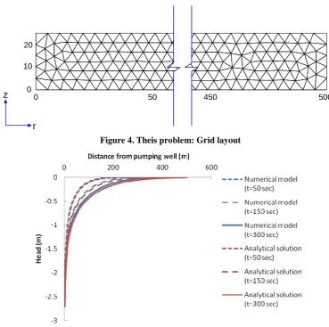
The computational mesh is shown in Fig.4. In Fig.5, the numerical and analytical solutions are compared. As illustrated in Fig. 5, numerical results closely correspond to the analytical solutions.
Figure 4. Theis problem: Grid layout
Figure 5. Theis problem: comparison between numerical and analytical solutions
5. Conclusions
This study presents a mass conservative method to model the axisymmetric groundwater flow toward a pumping well. Since the MPFA methods use head values in more than two cells in the unstructured grids, applying this scheme improves the accuracy of the result.
0 450 500
0 10 20
r
Furthermore, the diamond method has been implemented to construct the flux expression in terms of head values at the vertices and cell centers. Moreover, to interpolate the hydraulic values at the vertices, the least square method has been applied. Finally, to investigate the efficiency of the proposed numerical scheme, the model is verified against the Theis solution as a milestone in well hydraulics. The result illustrates that the model successfully simulates the transient drawdown in the confined aquifers.
References
1. Theis CV (1935) The relation between the lowering of the piezometric surface and the rate and duration of discharge of a well using ground-water storage. Transactions American Geophysical Union, 16, 519–24.
2. Hantush, MS, Jacob CE (1955) Non-steady radial flow in an infinite leaky aquifer. Eos, Transactions American Geophysical Union, 36(1), 95-100.
3. Neuman SP (1972) Theory of flow in unconfined aquifers considering delayed gravity response. Water Resources Research 8(4), 1031–1045.
4. Neuman SP (1973) Supplementary comments on theory of flow in unconfined aquifers considering delayed gravity response. Water Resources Research 9(4), 1102–1103.
5. Neuman SP (1974) Effect of partial penetration on flow in unconfined aquifers considering delayed gravity response. Water Resources Research 10(2), 303–312.
6. Neuman SP (1975) Analysis of pumping test data from anisotropic unconfined aquifers. Water Resources Research, 11(2), 329–345.
7. Vermeer PA, Verruijt A (1981) An accuracy condition for consolidation by finite elements. International Journal of Numeical and Analytical Methods in Geomechanics, 5(1), 1-14.
8. Murad MA, Loula AFD (1992) Improved accuracy in finite element analysis of Biot’s consolidation problem. Computer Methods in Applied Mechanics and Engineering 95(3), 359–382.
9. Ferronato M, Castelletto N, Gambolati G (2010) A fully coupled 3-D mixed finite element model of Biot consolidation. Journal of Computational Physics, 229(12), 4813–4830.
10. Kim J (2010) Sequential methods for coupled geomechanics and multiphase flow. PhD thesis, Stanford University.
11. Asadi R, Ataie-Ashtiani B (2015) A comparison of finite volume formulations and coupling strategies for two-phase flow in deforming porous media. Computers and Geotechnics, 67, 17-32.
12. Asadi R, Ataie-Ashtiani B, Simmons CT (2014) Finite volume coupling strategies for the solution of a Biot consolidation model. Computers and Geotechnics, 55, 494-505.
13. Asadi R, Ataie-Ashtiani B (2016) Numerical modeling of subsidence in saturated porous media: A mass conservative method. Journal of hydrology, 542, 423-436.
15. Manzini G, Ferraris S (2004) Mass-conservative finite volume methods on 2-D unstructured grids for the Richards’ equation. Advances in Water Resources, 27(12), 1199-1215.
16. Lee SH, Jenny P, Tchelepi HA (2002) A finite-volume method with hexahedral multiblock grids for modeling flow in porous media. Computers and Geosciences, 6(3-4), 353-379.
17. Edwards MG (2002) Unstructured, control-volume distributed, full-tensor finite-volume schemes with flow based grids. Computational Geosciences, 6(3-4), 433-452.
18. Szymkiewicz A (2012) Modelling water flow in unsaturated porous media: accounting for nonlinear permeability and material heterogeneity. Springer Science & Business Media.
19. Coudière Y, Villedieu P (2000) Convergence rate of a finite volume scheme for the linear convection-diffusion equation on locally refined meshes. Mathematical Modelling and Numerical Analysis, 34(6), 1123-1149.
20. Coudière Y, Vila JP, Villedieu P (1999) Convergence rate of a finite volume scheme for a two dimensional convection–diffusion problem, Mathematical Modelling and Numerical Analysis, 33, 493–516.
21. Bertolazzi E, Manzini G (2004) A cell-centered second-order accurate finite volume method for convection–diffusion problems on unstructured meshes. Mathematical Models and Methods in Applied Sciences, 14(8), 1235-1260.
22. Bertolazzi E, Manzini G (2005) A unified treatment of boundary conditions in least-square based finite-volume methods. Computers & Mathematics with Applications, 49(11), 1755-1765.
23. Bevilacqua I, Canone D, Ferraris S (2011) Acceleration techniques for the iterative resolution of the Richards equation by the finite volume method. International Journal for Numerical Methods in Biomedical Engineering, 27(8), 1309-1320.
24. Biot MA (1941) General theory of three-dimensional consolidation. Journal of Applied Physics, 12, 155–164.
25. Edwards MG, Rogers C (1998) Finite volume discretization with imposed flux continuity for the general tensor pressure equation. Computers & Geosciences, 2(4), 259–290.
26. Schöberl J (1997) NETGEN An advancing front 2D/3D-mesh generator based on abstract rules. Computing and Visualization in Science, 1(1), 41-52.
27. Fetter CW (1994) Applied Hydrogeology, third ed. Prentice Hall, New Jersey.
28. Bedient PB, Rifai HS, Newell CJ (1994). Ground water contamination: transport and remediation. Prentice-Hall International, Inc.