Determination of Location of FACTS Devices
using Sensitivity Index
Jyoti Saraswat1, Ankush Kumar Sharma2
Assistant Professor, Dept. of EE, Baddi University of Emerging Sciences &Technology, Baddi, H.P, India1
M.Tech Student [PE&D],Dept. of EE, Baddi University of Emerging Sciences &Technology, Baddi, H.P, India2
ABSTRACT:Power flow analysis is a necessary tool for power system designing, operation, planning, control and its economic scheduling. It gives information about the voltage, power angle, active and reactive power flow in the transmission lines and losses, using these parameters necessary steps can be taken to mitigate power quality issues. In this load flow is analysed using Newton – Raphson and Gauss – Seidel for IEEE 30 bus system. The voltage and angle find out using load flow is used for locating the optimal location for FACTS device.
With the increase of demand, the transmission lines operates at their stability limits. If the demand is further increased the transmission line gets congested and unable to fulfil that increased demand or system may collapse. For this, we use Flexible AC transmission system devices, since they can increase the usage capability of transmission system by controlling power flow in the network. In this paper location for FACTS device is find out using reduction of total system VAR power losses.
KEYWORDS:Load flow, Newton – Raphson, Gauss – Seidel, Sensitivity analysis, FACTS
I.INTRODUCTION
Load flow study in power system is the steady state solution of the power system network. The power system is modelled by an electric network and solved for the steady-state powers and voltages at various buses. The direct analysis of the circuit is not possible as the load are given in terms of complex power rather than impedances and the generators behave more like power sources than voltage sources[5].
Power flow studies, commonly referred to as load flow, are the backbone of power system analysis and design. They are necessary for planning, operation, economic scheduling and exchange of power between utilities. They are also suitable for analyses such as transient stability and contingency studies [6].
In solving a power flow problem the system is assumed to be operating under balanced condition and a single phase model is used [6]. The load flow analysis gives the information about active, reactive power flow, magnitudes and phase angle of voltages at each bus. The system buses are of following types:-
(i) Slack bus or swing bus: - In this, magnitude and phase angle of bus is specified.
(ii) Load bus: - In this, active and reactive power are specified. The magnitude and phase angle of bus voltage is unknown. These buses are also called as PQ bus.
(iii)Regulated bus: - In this bus, active power and voltage magnitude are specified. These bus are also called as generator bus or PV bus.
The state of power system and the methods of calculating this state are very important in evaluating the operation and control of power system and determination of future expansion for this system. The state of any power system can be determined using load flow analysis that calculates the power flowing through the lines of the system. Developments have been made in finding digital computer solutions for power-system load flows. This involves increasing the reliability and the speed of convergence of the numerical-solution techniques. There are different methods to determine the load flow for a particular system such as Gauss-Seidel, Newton-Raphson and Fast decoupled methods [6].
II.POWER FLOW EQUATIONS
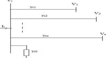
Consider a system having n buses as shown in Fig. 1.The transmission lines are represented by their equivalent network where impedances are converted into per unit admittances on a common MVA base. By applying KVL to the system we get equations for bus voltages and equation for power flowing.
Fig. 1 A n bus system in power system Applying KVL to this bus system:
Ii = yi0Vi0 + yi1 ( Vi – V1 ) + yi2 ( Vi – V2 ) +………. + yin ( Vi – Vn )
= (yi0 + yi1 + yi2 + …+ yin ) Vi - yi1 V1 - yi2 V2 - . . . - yin Vn (1)
Ii = Vi∑ - ∑ Vj i ≠ j (2)
Where,
Ii = current flowing in bus i
Vi = voltage at bus i
V1 , V2 , . . . Vn are the voltages at buses 1 , 2 , . . . n respectively
Now, active and reactive power flowing at bus i is given as: Pi + jQi = Vi ∗
Ii =
∗ (3)
Putting the value of Ii from 1.2 in equation 1.3 getting equation as:
∗ = Vi∑ - ∑ Vj (4)
So these are the equations involved for active and reactive power flowing from buses 1 to n
Power flow solution using Gauss–Seidel analysis
Gauss–Seidel is the iterative method for calculating the variables involved in load flow flow analysis. It is used because of its simplicity in solving the load flow calculations. In load flow analysis a set of equations are solved for two unknown variables at each node. In GS method the iterative sequence for calculation of Vi for equation 4 is given as:
V = ∗
∑
∑ (5)
Where,
yij = admittance in per unit
Pish= active power in per unit flowing through transmission line
Qish = reactive power in per unit flowing through transmission line
For PV buses Pish and Qish have positive values because power is flowing in the bus and for PQ buses Pish and Qish have
negative values because the power is flowing away from the bus. The iterative solution for active and reactive power flow is given as:
Pik+1 = R { Vi*k [ Vik∑ y - ∑ y V ]}j ≠ i (6)
Qik+1 = - I { Vi*k [ Vik∑ y - ∑ y V ]} j ≠ i (7)
For PQ bus Pish and Qish is known, it is used to solve equation 1.8 from that phase angle and voltage magnitude is
calculated. For PV bus Pish and | Vi | are known and equation 7 is solved for Qik+1, this calculated value is used to solve
equation 5 , after solving voltage angle is calculated and voltage magnitude remain same.
The iteration process continues until the convergence occurs criteria is not specified. The convergence criteria is given as:
|∆ Vik+1| = | Vik+1| - | Vik+1| ≤ ɛ (8)
Power flow solution using Newton- Raphson analysis
Newton Raphson is quadratic in convergence and is less prone to divergence with ill conditioned problems. So it is superior to G-S method. The numbers of iteration required to obtain the solution is independent to the size of network but more functional evaluations are required at each iterations. The newton Raphson is written in polar form. From equation 2 current entering at bus i is given as [6]:
Ii = ∑ Y Vj (9)
By writing this equation in polar form
Ii = ∑ |Y | |Vj |∠θij + δj (10)
The complex power flowing at bus i is given as
Pi – jQi = Vi*Ii (11)
By putting the value of Ii in equation 11
Pi – jQi = | Vi | ∠-δi∑ |Y | |Vj |∠θij + δj (12)
After separating real and imaginary parts equation 12 becomes
Pi = ∑ |Y | |Vj | |Vi | cos(θ − δi +δj ) (13)
Qi = -∑ |Y | |Vj | |Vi | sin(θ - δi +δj ) (14)
By expanding non-linear equations 13 and 14 using Taylor’s series about all initial estimates and neglecting all higher order terms results in following sets of linear equations[8],[9].
⎣ ⎢ ⎢ ⎢ ⎡∆... ∆ ∆ .. . ∆ ⎦ ⎥ ⎥ ⎥ ⎤ = ⎣ ⎢ ⎢ ⎢ ⎢ ⎢ ⎢ ⎡ ⎝ ⎜ ⎛ ⋯ ⋮ ⋱ ⋮ ⋯ ⎠ ⎟ ⎞ ⎝ ⎜ ⎛ ⋯ ⋮ ⋱ ⋮ ⋯ ⎠ ⎟ ⎞ ⎝ ⎜ ⎛ | | ⋯ | | ⋮ ⋱ ⋮ | | ⋯ | |⎠ ⎟ ⎞ ⎝ ⎜ ⎛ | | ⋯ | | ⋮ ⋱ ⋮ | | ⋯ | |⎠ ⎟ ⎞ ⎦ ⎥ ⎥ ⎥ ⎥ ⎥ ⎥ ⎤ ⎣ ⎢ ⎢ ⎢ ⎡∆... ∆ ∆| | .. . ∆| |⎦ ⎥ ⎥ ⎥ ⎤
The bus is supposed to be a slack bus. The elements of Jacobian matrix are the partial derivative of equations 13 and 14. It gives the relationship between the small change in voltage angles ∆δik and voltage magnitude ∆| Vik | with small
change in active and reactive power ∆Pik and ∆Qik.In short the Jacobian matrix can written as:
∆P
∆Q =
J J
J J
∆δ
∆|V| (15)
For voltage controlled buses voltage magnitudes are known. If there are m voltage controlled buses then there are m equations which have to solved for ∆Q and ∆V and accordingly the coloumns of jacobian matrix is neglected. If there are n buses then n-1 active power constraints (n – 1– m) reactive power constraints. The jacobian matrix is of the order of (2n – 2 – m) × (2n – 2 – m).
The diagonal and off diagonal elements of J1 are written as
= ∑ |Y | |Vj | |Vi | sin (θ - δi +δj) j ≠ i (16)
= - | Vi | | Vj | |Yij | sin (θ - δi +δj) j ≠ i (17)
The diagonal and off diagonal elements of J2 are written as:
| | = 2 | Vi | | Yii | cos(θ ) + ∑ |Y | |Vj |cos(θ - δi +δj ) j ≠ i (18)
| | = | Vi | | Yij | cos(θ - δi +δj ) j ≠ i (19)
The diagonal and off diagonal elements of J3 are written as
= - | Vi | | Vj | |Yij | cos(θ - δi +δj ) j ≠ i ( 21 )
The diagonal and off diagonal elements of J4 are written as:
| | = - 2 | Vi | | Yii | sin(θ ) – ∑ |Y | |Vj | sin(θ - δi +δj ) j ≠ i (22)
| | = - | Vi | | Yij | sin(θ - δi +δj ) j ≠ i (23)
Also, the mismatch between the scheduled power and calculated power is given as[10]:
∆Pik = Pish – Pik (24)
∆Qik = Qish – Qik (25)
Where Pish , Qish are the scheduled active and reactive power
Pik , Qik are the calculated active and reactive power
∆Pik = mismatch in active power
∆Qik = mismatch in reactive power
So by knowing the values of mismatches in power and Jacobian matrix,the change in voltage magnitude and voltage angle is calculated by the equation as:
∆δ ∆|V| =
J J
J J
∆P
∆Q (26)
The updated values of voltage magnitude and voltage angle are given as:
δ = δ + ∆δ (27)
| Vik+1 | = | Vik | + ∆| Vik | (28)
The updating continues until the mismatch were less than some prespecified value.
| ∆Pik | ≤ ɛ and | ∆Qik | ≤ ɛ (29)
III.LOCATION OF FACTS DEVICE
The location of FACTS device is determined using reduction of total system reactive power loss. It is based on the sensitivity of the total system reactive power loss with respect to control variable of the FACTS device. For placement of FACTS device between buses i and j net line series reactance is taken as control variable. Loss sensitivity with respect to control parameter of FACTS placed between ith and jth bus is given as [1],[2]:
aij = (30)
= [ Vi2 + Vj2 – 2ViVjcos ( δij ) ] × {
–
( – ) } (31)
IV.RESULTS AND DISCUSSION
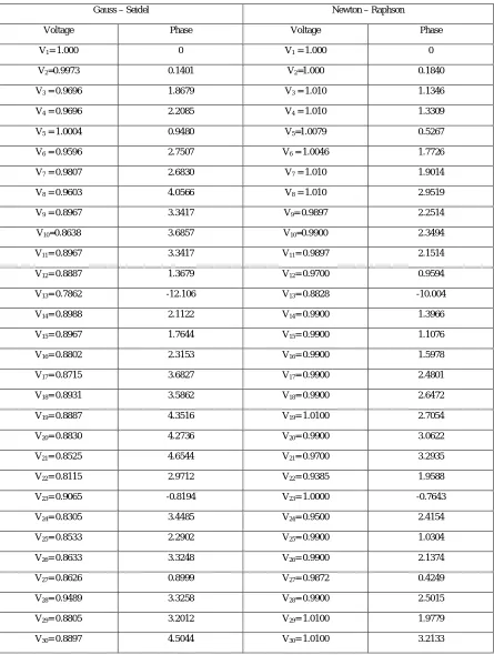
Table IVoltage and Phase angle for IEEE 30 bus system
Gauss – Seidel Newton – Raphson
Voltage Phase Voltage Phase
V1= 1.000 0 V1 = 1.000 0
V2=0.9973 0.1401 V2=1.000 0.1840
V3 = 0.9696 1.8679 V3 = 1.010 1.1346
V4 = 0.9696 2.2085 V4 = 1.010 1.3309
V5 = 1.0004 0.9480 V5=1.0079 0.5267
V6 = 0.9596 2.7507 V6 = 1.0046 1.7726
V7 = 0.9807 2.6830 V7 = 1.010 1.9014
V8 = 0.9603 4.0566 V8 = 1.010 2.9519
V9 = 0.8967 3.3417 V9= 0.9897 2.2514
V10=0.8638 3.6857 V10=0.9900 2.3494
V11= 0.8967 3.3417 V11= 0.9897 2.1514
V12= 0.8887 1.3679 V12= 0.9700 0.9594
V13= 0.7862 -12.106 V13= 0.8828 -10.004
V14= 0.8988 2.1122 V14= 0.9900 1.3966
V15= 0.8967 1.7644 V15= 0.9900 1.1076
V16= 0.8802 2.3153 V16= 0.9900 1.5978
V17= 0.8715 3.6827 V17= 0.9900 2.4801
V18= 0.8931 3.5862 V18= 0.9900 2.6472
V19= 0.8887 4.3516 V19= 1.0100 2.7054
V20= 0.8830 4.2736 V20= 0.9900 3.0622
V21= 0.8525 4.6544 V21= 0.9700 3.2935
V22= 0.8115 2.9712 V22= 0.9385 1.9588
V23= 0.9065 -0.8194 V23= 1.0000 -0.7643
V24= 0.8305 3.4485 V24= 0.9500 2.4154
V25= 0.8533 2.2902 V25= 0.9900 1.0304
V26= 0.8633 3.3248 V26= 0.9900 2.1374
V27= 0.8626 0.8999 V27= 0.9872 0.4249
V28= 0.9489 3.3258 V28= 0.9900 2.5015
V29= 0.8805 3.2012 V29= 1.0100 1.9779
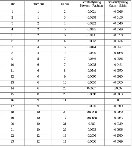
The table II shows the sensitivity analysis of system, it is done after the load flow is over. The bus voltage and phase angle which are obtained from load flow analysis is used in sensitivity analysis. The sensitivity analysis is done by calculating total system reactive power loss with respect to series reactance of the line. The sensitivity analysis is done through Gauss -Seidel and Newton – Raphson method and optimal location of FACTS device is find out. The FACTS devices are to be placed where the sensitivity is most negative and have positive values because these are the places if a FACTS device is placed there, it will decrease the net series reactance of the transmission line and active power transfer capability of line is increased.
Table IISensitivity using Newton – Raphson and Gauss – Seidel for IEEE 30 bus system
Line From bus To bus Sensitivityusing
Newton – Raphson
Sensitivity using Gauss – Seidel
1 1 2 -0.0021 -0.0026
2 1 3 -0.0103 -0.0406
3 2 4 -0.0112 -0.0546
4 2 5 -0.0245 -0.0519
5 2 6 -0.0176 -0.0758
6 3 4 -0.0062 -0.0424
7 4 6 -0.0464 -0.0477
8 4 12 -0.0310 -0.1068
9 5 7 -0.0246 -0.0536
10 6 7 -0.0035 -0.0461
11 6 8 -0.0546 -0.0570
12 6 9 -0.0060 -0.0910
13 6 10 -0.0010 -0.0300
14 6 28 0.0067 0.0037
15 8 28 -0.0088 -0.0053
16 9 11 0 0
17 9 10 -0.0010 -0.0919
18 10 20 -0.00200 -0.0060
19 10 17 -0.00050 -0.0053
20 10 21 -0.682 -0.0349
21 10 22 -0.0633 -0.0666
22 12 13 -0.2006 -0.2530
24 12 15 -0.0103 -0.0026
25 12 16 -0.0353 -0.0194
26 14 15 0.0002 0.00030
27 15 18 -0.0070 -0.0082
28 15 23 -0.0135 -0.0204
29 16 17 -0.0038 -0.0082
30 18 19 -0.0127 -0.0051
31 19 20 -0.0522 -0.0040
32 21 22 -0.0306 -0.0467
33 22 24 -0.0019 -0.0042
34 23 24 -0.0377 -0.0691
35 24 25 -0.0074 -0.0028
36 25 26 -0.0007 -0.0007
37 25 27 -0.0012 -0.0053
38 27 29 -0.0032 -0.0040
39 27 30 -0.0035 -0.0045
40 28 27 -0.0081 -0.0557
41 29 30 -0.0012 -0.0013
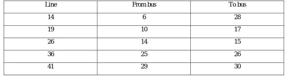
The table III shows the location of FACSTS devices after analysis from table II. The optimal location are the values where sensitivity have positive or most negative value or close to zero.
Table III Optimal location for FACTS device for IEEE 30 bus system
Line From bus To bus
14 6 28
19 10 17
26 14 15
36 25 26
41 29 30
V. CONCLUSION
From the present work it can be inferred that Newton – Raphson method is better than Gauss –Seidel method in finding the load flow solution. The N – R takes lesser numbers of iterations as comparison to Gauss – Seidel. As the numbers of buses increases the numbers of iterations for G – S increases and if we further increases the number of buses the Gauss – Seidel may diverge in some cases. The calculation used in Gauss – Seidel are simple whereas in Newton – Raphson method the calculation is difficult for Jacobian matrix, it is most time consuming in N – R. The Newton – Raphson method may diverge in some cases if Jacobian matrix becomes singular, so its singularity has to be removed. Also, the optimal location findings using N – R are better than Gauss – Seidel method because G – S may diverge if system requires higher accuracy and high bus number. The numbers of optimal locations increases as the bus number increases. So the optimal location for FACTS device is points where sensitivity are positive and close to origin.
VI. FUTURE SCOPE
The proposed work is done to find out the load flow and then optimal location for FACTS device. In future the work can be extended to design the control scheme of FACTS devices and find its operating characteristics, so that it can be placed in the transmission line, finding its effect on the active power flowing through the line, its effect on the transient behaviour on the line and other other effects. In future other FACTS devices such as UPFC, TCSR can be studied for their optimal location and control characteristics.
REFERENCES
[1] L.Rajalakshmi,M.V. Suganyadevi, S. Parameswari, “CongestionManagement in Deregulated Power System by Locating Series FACTS Devices,” International Journal of Computer Applications, Vol. 13, 2011
[2] Sunil Malival, Y.R. Prajapati, “Optimal Location and Cost Analysis of TCSC for Improving Power System Stablility and Economy,” International Journal ofAdvance Engineering andResearch Development, Vol. 1, 2014
[3] J. Teng, “A Modified Gauss SeidelAlgorithm of Three-Phase Power Flow Analysis in Distribution Networks,” Electric Power and Energy Systems, Vol. 24, pp. 2–7, 2002.
[4] T. Kulworawanichpong, “Electrical Power and Energy Systems Simplified Newton – Raphson Power-Flow Solution Method,” International Journal of Electrical Power and Energy Systems, Vol. 32, No. 6, pp. 551–558, 2010.
[5] D.P.Kothari,I.J Nagrath,”Modern Power System Analysis”, Mcgraw-Hill; 2003 [6] Saadat H. “Power System Analysis”, Mcgraw-Hill; 2004.
[7] N. G. Hingaroni and L. Gyugyi, “Understanding FACTS Concepts and Technology of Flexible Ac Transmission System,” IEEE Press, New York, 2000
[8] H. Le Nguyen, “Newton– Raphson Method in Complex Form,” IEEE Transaction on Power Systems, Vol. 12, pp. 1355- 1359, 1997 [9] D. K. Tanti, “Load Flow Analysis on IEEE 30 Bus System,” International Journal of Scientific and Research Publication, Vol. 2, No. 11,
pp. 1–6, 2012.