A Self-Localization Method for Wireless
Sensor Networks
Randolph L. Moses
Department of Electrical Engineering, The Ohio State University, 2015 Neil Avenue, Columbus, OH 43210, USA Email:[email protected]
Dushyanth Krishnamurthy
Department of Electrical Engineering, The Ohio State University, 2015 Neil Avenue, Columbus, OH 43210, USA
Robert M. Patterson
Department of Electrical Engineering, The Ohio State University, 2015 Neil Avenue, Columbus, OH 43210, USA Email:[email protected]
Received 30 November 2001 and in revised form 9 October 2002
We consider the problem of locating and orienting a network of unattended sensor nodes that have been deployed in a scene at unknown locations and orientation angles. This self-calibration problem is solved by placing a number of source signals, also with unknown locations, in the scene. Each source in turn emits a calibration signal, and a subset of sensor nodes in the network measures the time of arrival and direction of arrival (with respect to the sensor node’s local orientation coordinates) of the signal emitted from that source. From these measurements we compute the sensor node locations and orientations, along with any unknown source locations and emission times. We develop necessary conditions for solving the self-calibration problem and provide a maximum likelihood solution and corresponding location error estimate. We also compute the Cram´er-Rao bound of the sensor node location and orientation estimates, which provides a lower bound on calibration accuracy. Results using both synthetic data and field measurements are presented.
Keywords and phrases:sensor networks, localization, location uncertainty, Cram´er-Rao bound.
1. INTRODUCTION
Unattended sensor networks are becoming increasingly im-portant in a large number of military and civil applications [1,2,3,4]. The basic concept is to deploy a large number of low-cost self-powered sensor nodes that acquire and process data. The sensor nodes may include one or more acoustic mi-crophones as well as seismic, magnetic, or imaging sensors. A typical sensor network objective is to detect, track, and clas-sify objects or events in the neighborhood of the network.
We consider a sensor deployment architecture as shown in Figure 1. A number of low-cost sensor nodes, each equipped with a processor, a low-power communication transceiver, and one or more sensing capabilities, are set out in a planar region. Each sensor node monitors its environ-ment to detect, track, and characterize signatures. The sensed data is processed locally, and the result is transmitted to a lo-cal central information processor (CIP) through a low-power communication network. The CIP fuses sensor information and transmits the processed information to a higher-level processing center.
Central information
processor Higher-level
processing center
Sensors
Figure1: Sensor network architecture. A number of low-cost sen-sor nodes are deployed in a region. Each sensen-sor node communicates to a local CIP, which relays information to a more distant command center.
Array 2 (x2, y2)
θ2
SourceS
( ˜xS,˜yS) ArrayA
(xA, yA)
θA
Source 1 ( ˜x1,y1˜)
Array 1
(x1, y1)
θ1
Figure2: Sensor self-localization scenario.
launch. For careful hand placement, accurate location and orientation of the sensor nodes can be assumed; however, for most other sensor deployment methods, it is difficult or im-possible to know accurately the location and orientation of each sensor node. One could equip every sensor node with a GPS and compass to obtain location and orientation infor-mation, but this adds to the expense and power requirements of the sensor node and may increase susceptibility to jam-ming. Thus, there is interest in developing methods to self-localize the sensor network with a minimum of additional hardware or communication.
Self-localization in sensor networks is an active area of current research (see, e.g., [1,5,6,7,8] and the references therein). Iterative multilateration-based techniques are con-sidered in [7], and Bulusu et al. [5, 9] consider low-cost localization methods. These approaches assume availability of beacon signals at known locations. Sensor localization, coupled with near-field source localization, is considered in [10,11]. Cevher and McClellan consider sensor network self-calibration using a single acoustic source that travels along a straight line [12]. The self-localization problem is also re-lated to the calibration of element locations in sensor arrays [13,14,15,16,17,18]. In the element calibration problem, we assume knowledge of the nominal sensor locations and assume high (or perfect) signal coherence between the sen-sors; these assumptions may not be satisfied for many sensor network applications, however.
In this paper, we consider an approach to sensor network self-calibration using sources at unknown locations in the field. Thus, we relax the assumption that beacon signals at known locations are available. The approach entails placing a number of signal sources in the same region as the sensor nodes (seeFigure 2). Each source in turn generates a known signal that is detected by a subset of the sensor nodes; each sensor node that detects the signal measures the time of ar-rival (TOA) of the source with respect to an established net-work time base [19,20] and also measures the direction of ar-rival (DOA) of the source signal with respect to a local (to the sensor node) frame of reference. The set of TOA and DOA
measurements are collected together and form the data used to estimate the unknown locations and orientations of the sensor nodes.
In general, neither the source locations nor their signal emission times are assumed to be known. If the source sig-nal emission times are unknown, then the time of arrival to any one sensor node provides no information for self-localization; rather, time difference of arrival (TDOA) be-tween sensor nodes carries information for localization. If partial information is available, it can be incorporated into the estimation procedure to improve the accuracy of the cali-bration. For example, [21] considers the case in which source emission times are known; such would be the case if the sources were electronically triggered at known times.
We show that if neither the source locations nor their signal emission times are known and if at least three sensor nodes and two sources are used, the relative locations and orientations of all sensor nodes, as well as the locations and signal emission times of all sources, can be estimated. The calibration is computed except for an unknown translation and rotation of the entire source-signal scene, which cannot be estimated unless additional information is available. With the additional location or orientation information of one or two sources, absolute location and orientation estimates can be obtained.
We consider optimal signal processing of the measured self-localization data. We derive the Cram´er-Rao bound (CRB) on localization accuracy. The CRB provides a lower bound on any unbiased localization estimator and is useful to determine the best-case localization accuracy for a given problem and to provide a baseline standard against which suboptimal localization methods can be measured. We also develop a maximum likelihood (ML) estimation procedure, and show that it achieves the CRB for reasonable TOA and DOA measurement errors.
There is a great deal of flexibility in the type of signal sources to be used. We require only that the times of arrival of the signals can be estimated by the sensor nodes. This can be accomplished by matched filtering or generalized cross-correlation of the measured signal with a stored waveform or set of waveforms [22,23]. Examples of source signals are short transients, FM chirp waveforms, PN-coded or direct-sequence waveforms, or pulsed signals. If the sensor nodes can also estimate signal arrival directions (as is the case with vector pressure sensors or arrays of microphones), these esti-mates can be used to improve the calibration solution.
2. PROBLEM STATEMENT AND NOTATION
Assume we have a set of A sensor nodes in a plane, each with unknown location{ai=(xi, yi)}Ai=1and unknown ori-entation angle θiwith respect to a reference direction (e.g., North). We consider the two-dimensional problem in which the sensor nodes lie in a plane and the unknown reference direction is azimuth; an extension to the three-dimensional case is possible using similar techniques. A sensor node may consist of one or more sensing element; for example, it could be a single sensor, a vector sensor [24], or an array of sensors in a fixed known geometry. If the sensor node does not mea-sure the DOA, then its orientation angleθiis not estimated.
In the sensor field are also placedSpoint sources at lo-cations{sj = (˜xj,y˜j)}Sj=1. The source locations are in gen-eral unknown. Each source emits a known finite-length sig-nal that begins at timetj; the emission times are also in gen-eral unknown.
Each source emits a signal in turn. Every sensor node at-tempts to detect the signal, and if detected, the sensor node estimates the TOA of the signal with respect to a sensor net-work time base, and a DOA with respect to the sensor node’s local reference direction. The time base can be established either by using the electronic communication network link-ing the sensor nodes [19,20] or by synchronizing the sen-sor node processen-sor clocks before deployment. The time base needs to be accurate to a number on the order of the time of arrival measurement uncertainty (1 ms in the examples con-sidered inSection 5). The DOA measurements are made with respect to a local (to the sensor node) frame of reference. The absolute directions of arrival are not available because the orientation angle of each sensor node is unknown (and is estimated in the calibration procedure). Both the TOA and DOA measurements are assumed to contain estimation er-rors. We denote the measured TOA at sensor nodeiof source
jasti jand the measured DOA asθi j.
We initially assume every sensor node detects ev-ery source signal; partial measurements are considered in Section 4.4. If so, a total of 2ASmeasurements are obtained. The 2ASmeasurements are gathered in a vector
X=
where vec(M) stacks the elements of a matrixMcolumnwise and where
Each sensor node transmits its 2STOA and DOA measure-ments to a CIP, and these 2ASmeasurements form the data with which the CIP computes the sensor calibration. Note that the communication cost to the CIP is low, and the cali-bration processing is performed by the CIP.
The above formulation implicitly assumes that sensor node measurements can be correctly associated to the corre-sponding source. That is, each sensor node TOA and DOA measurement corresponding to source j can be correctly attributed to that source. There are several ways in which this association can be realized. One method is to time-multiplex the source signals so that they do not overlap. If the source firing times are separated, then any sensor node detection within a certain time interval can be attributed to a unique source. Alternately, each source can emit a unique identifying tag, encoded, for example, in its transmitted sig-nal. In either case, failed detections can be identified at the CIP by the absence of a report from sensor node i about source j. Finally, we can relax the assumption of perfect as-sociation by including a data asas-sociation step in the self-localization algorithm, using, for example, the methods in [25,26].
Define the parameter vectors
β= x1, y1, θ1, . . . , xA, yA, θA
Note thatβcontains the sensor node unknowns andγ con-tains the source signal unknowns. We denote the true TOA and DOA of source signal j at sensor nodeiasτi j(α) and
φi j(α), respectively, and include their dependence on the pa-rameter vectorα; they are given by
τi j(α)=tj+
cis the signal propagation velocity.
Each element of X has measurement uncertainty; we model the uncertainty as
X=µ(α) +E, (5) whereµ(α) is the noiseless measurement vector whose ele-ments are given by (4) for values ofiand jthat correspond to the vector stacking operation in (1), and whereEis a ran-dom vector with known probability density function.
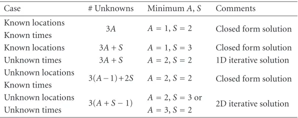
Table1: Minimal solutions for sensor self-localization.
Case # Unknowns MinimumA,S Comments
Known locations
3A A=1,S=2 Closed form solution Known times
Known locations 3A+S A=1,S=3 Closed form solution Unknown times 3A+S A=2,S=2 1D iterative solution Unknown locations
3(A−1)+2S A=2,S=2 Closed form solution Known times
Unknown locations
3(A+S−1) A=2,S=3 or 2D iterative solution Unknown times A=3,S=2
3. EXISTENCE AND UNIQUENESS OF SOLUTIONS
In this section, we address the existence and uniqueness of solutions to the self-calibration problem and establish the minimum number of sensor nodes and sources needed to obtain a solution. We assume that every sensor node detects every source and measures both TOA and DOA. In addi-tion, we assume that the TOA and DOA measurements are noiseless and correspond to values that correspond to a pla-nar sensor-source scepla-nario; that is, we assume they are solu-tions to (4) for some vectorα ∈ 3(A+S). We establish the minimum number of sources and sensor nodes needed to compute a unique calibration solution and give algorithms for finding the self-calibration solution in the minimal cases. These algorithms provide initial estimates to an iterative de-scent algorithm for the practical case of nonminimal noisy measurements presented inSection 4.
The four cases below make different assumptions on what is known about the source signal locations and emis-sion times. Of primary interest is the case where no source parameters are known; however, the solution for this case is based on solutions for cases in which partial information is available, so it is instructive to consider all four cases. In all four cases, the number of measurements is 2AS, and de-termination of βinvolves solving a nonlinear set of equa-tions for its 3Aunknowns. Depending on the case consid-ered, we may also need to estimate the unknown nuisance parameters in γ. The result in each case is summarized in Table 1.
Case 1 (known source locations and emission times). A unique solution forβcan be found for any number of sensor nodes as long as there are S ≥ 2 sources. In fact, the loca-tion and orientaloca-tion of each sensor node can be computed independently of other sensor node measurements. The lo-cation of theith sensor nodeai is found from the intersec-tion of two circles with centers at the source locaintersec-tions and with radii (ti1−t1)/cand (ti2−t2)/c. The intersection is in general two points; the correct location can be found us-ing the sign ofθi2−θi1. We note that the two circle inter-sections can be computed in closed form. Finally, from the known source and sensor node locations and the DOA mea-surements, the sensor node orientationθican be uniquely found.
ai
s2 s1
θi2−θ
i1
Figure3: A circular arc is the locus of possible sensor node loca-tions whose angle between two known points is constant.
Case 2 (known source locations and unknown emission times). For S ≥ 3 sources, the location and orientation of each sensor node can be computed in closed form inde-pendently of other sensor nodes. A solution procedure is as follows. Consider the pair of sources (s1, s2). Sensor nodei knows the angleθi2−θi1between these two sources. The set of all possible locations for sensor nodeiis an arc of a circle whose center and radius can be computed from the source locations (seeFigure 3). Similarly, a second circular arc is ob-tained from the source pair (s1, s3). The intersection of these two arcs is a unique point and can be computed in closed form. Once the sensor node location is known, its orienta-tionθiis readily computed from one of the three DOA mea-surements.
A solution for Case 2 can also be found using S = 2 sources andA=2 sensor nodes. The solution requires a one-dimensional search of a parameter over a finite interval. The known location ofs1 ands2and the known angleθ11−θ12 means that sensor node 1 must lie on a known circular arc as inFigure 3. Each location along the arc determines the source emission timest1andt2. These emission times are consistent with the measurements from the second sensor node for ex-actly one positiona1along the arc.
change theti j andθi j measurements. To eliminate this am-biguity, we assume that the location and orientation of the first sensor node are known; without loss of generality, we setx1 = y1 =θ1 =0. We solve for the remaining 3(A−1) parameters inβ.
For the case of unknown source locations, a unique so-lution forβis computable in closed form forS=2 and any
A ≥2 (the caseA= 1 is trivial). The range to each source from sensor node 1 can be computed fromrj =(t1j−tj)/c, and its bearing is known, so the locations of the two sources can be found. The locations and orientations of the remain-ing sensor nodes are then computed usremain-ing the method of Case 1.
Case4 (unknown source locations and emission times). For this case, it can be shown that an infinite number of calibra-tion solucalibra-tions exist forA =S = 2,1 but a unique solution exists in almost all cases for eitherA=2 andS=3 orA=3 andS=2. In some degenerate cases, not all of theγ param-eters can be uniquely determined, although we do not know a case for which theβparameters cannot be uniquely found. Closed form calibration solutions are not known for this case, but solutions that require a two-dimensional search can be found. We outline one such solution that works for either
A=2 andS≥3 orS=2 andA≥3. Assume as before that sensor node 1 is at location (x1, y1)=(0,0) with orientation
θ1=0. If we know the two source emission timest1andt2, we can find the locations of sources s1ands2 as inCase 3. From the two known source locations, all remaining sensor node locations and orientations can be found using the pro-cedure inCase 1, and then all remaining source locations can be found using triangulation from the known arrival angles and known sensor node locations. These solutions will be in-consistent except for the correct values oft1andt2. The cal-ibration procedure, then, is to iteratively adjustt1andt2to minimize the error between computed and measured time delays and arrival angles.
4. MAXIMUM LIKELIHOOD SELF-CALIBRATION
In this section, we derive ML estimator for the unknown sen-sor node location and orientation parameters.
The ML algorithm involves the solution of a set of nonlinear equations for the unknown parameters, includ-ing the unknown nuisance parameters inγ. The solution is found by iterative minimization of a cost function; we use the methods in Section 3to initialize the iterative descent. In addition, we derive the CRB for the variance of the un-known parameters inα; the CRB also gives parameter vari-ance of the ML parameter estimates for high signal-to-noise ratio (SNR).
The ML estimator is derived from a known parametric form for the measurement uncertainty inX. In this paper, we
1Note that forA=S=2, there are 8 measurements and 9 unknown
pa-rameters. The set of possible solutions in general lies on a one-dimensional manifold in the 9-dimensional parameter space.
adopt a Gaussian uncertainty. The justification is as follows. First, for sufficiently high SNR, TOA estimates obtained by generalized cross-correlation are Gaussian distributed with negligible bias [23]. The variance of the Gaussian TOA error can be computed from the signal spectral characteristics [23]. For broadband signals with flat spectra, the TOA error stan-dard deviation is roughly inversely proportional to the sig-nal bandwidth [21]. Furthermore, most DOA estimates are also Gaussian with negligible bias for sufficiently high SNR [27]. For single sources, the DOA standard deviation is pro-portional to the array beamwidth [28]. Thus, Gaussian TOA and DOA measurement uncertainty model is a reasonable as-sumption for sufficiently high SNR.
4.1. The maximum likelihood estimate
Under the assumption that the measurement uncertaintyE
in (5) is Gaussian with zero mean and known covarianceΣ, the likelihood function is
f(X;α)= 1 A special case is when the measurement errors are uncorre-lated and the TOA and DOA measurement errors have vari-ancesσt2andσθ2, respectively; (7) then becomes
Depending on the particular knowledge about the source sig-nal parameters, none, some, or all of the parameters inαmay be known. We letα1denote vector of unknown elements of
αand letα2denote the vector of known elements inα. Using
4.2. Nonlinear least squares solution
Equation (9) involves solving a nonlinear least squares prob-lem. A standard iterative descent procedure can be used, ini-tialized using one of the solutions inSection 3. In our imple-mentation, we used the Matlab functionlsqnonlin.
iterations if the methods are tuned appropriately. Similarly, one can view the source parameters as nuisance parameters and employ estimate-maximize (EM) algorithms to obtain the ML solution [30].
4.3. Estimation accuracy
The CRB gives a lower bound on the covariance of any unbi-ased estimate ofα1. It is a tight bound in the sense that ˆα1,ML has parameter uncertainty given by the CRB for high SNR; that is, as maxiΣii → 0. Thus, the CRB is a useful tool for analyzing calibration uncertainty.
The CRB can be computed from the Fisher information matrix ofα1. The Fisher information matrix is given by [22],
Iα1=E ∇α1lnf(T,Θ;α) ∇α1lnf(T,Θ;α)
T
. (10) The partial derivatives are readily computed from (6) and (4); we find that
For Cases3and4, the Fisher information matrix is rank deficient due to the translational and rotational ambiguity in the self-calibration solution. In order to obtain an invertible Fisher information matrix, some of the sensor node or source parameters must be known. It suffices to know the location and orientation of a single sensor node, or to know the lo-cations of two sensor nodes or sources. These assumptions might be realized by equipping one sensor node with a GPS and a compass, or by equipping two sensor nodes or sources with GPSs. Let ˜α1 denote the vector obtained by removing these assumed known parameters fromα1. To compute the CRB matrix for ˜α1in this case, we first remove all rows and columns in Iα1 that correspond to the assumed known
pa-rameters then invert the remaining matrix [22],
Cα˜1= Iα˜1 −1
. (12)
4.4. Partial measurements
So far we have assumed that every sensor node detects and measures both the TOA and DOA from every source signal. In this section, we relax that assumption. We assume that each emitted source signal is detected by only a subset of the sensor nodes in the field and that a sensor node that de-tects a source may measure the TOA and/or the DOA for that source, depending on its capabilities. We denote the availabil-ity of a measurement using two indicator functionsIt
i jandIi jθ, where
Ii jt, Ii jθ ∈ {0,1}. (13) If sensor nodeimeasures the TOA (DOA) for sourcej, then
It
i j = 1 (Ii jθ =1); otherwise, the indicator function is set to zero. Furthermore, letLdenote the 2AS×1 vector whosekth element is 1 ifXkis measured and is 0 ifXkis not measured;
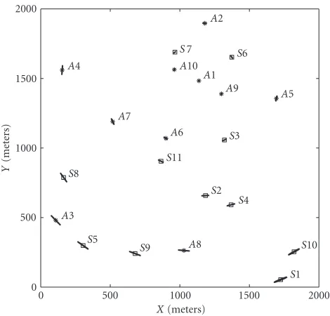
Figure 4: Example scene showing ten sensor nodes (stars) and eleven sources (squares). Also are shown the 2σlocation uncertainty ellipses of the sensor nodes and sources; these are on average less than 1 m in radius and show as small dots. The locations of sensor nodesA1 andA2 are assumed to be known.
stacking their columns into a vector as in (1). Finally, define ˜
Xto be the vector formed from elements ofXfor which mea-surements are available, soXkis in ˜XifLk=1.
The ML estimator for the partial measurement case is similar to (9) but uses only those elements ofX for which the corresponding element ofLis one. Thus,
ˆ
α1,ML=arg minα
1
˜
QX˜;α, (14)
where (assuming uncorrelated measurement errors as in (8)),
The Fisher information matrix for this case is similar to (11), but includes only information from available measurements; thus
111 110 109 108 107 106 105
X(meters) 477
478 479 480 481 482 483
Y
(met
ers)
A3
1300 1299
1298
X(meters) 1388
1389 1390
Y
(met
ers)
A9
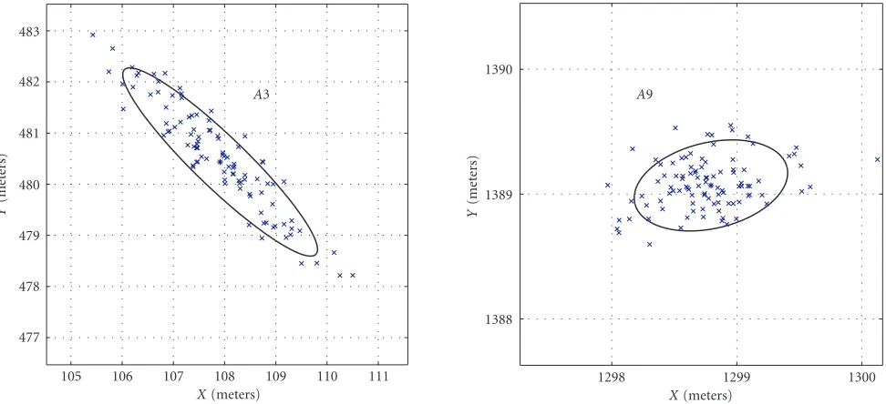
Figure5: Two standard deviation location uncertainty ellipses for sensor nodesA3 andA9 fromFigure 4.
Iα1= G
α 1
TΣ−1P D G
α1
, (18) wherePDis a diagonal matrix whosekth diagonal element is the probability that measurementXkis available.
We note that when partial measurements are available, the ML calibration may not be unique. For example, if only TOA measurements are available, a scene calibration solution and its mirror image have the same likelihoods. A complete understanding of the uniqueness properties of solutions in the partial measurement case is a topic of current research.
5. NUMERICAL RESULTS
This section presents numerical examples of the self-calibration procedure. First, we present a synthetically gener-ated example consisting of ten sensor nodes and 2–11 sources placed randomly in a 2 km×2 km region. Second, we present results from field measurements using four acoustic sensor nodes and four acoustic sources.
5.1. Synthetic data example
We consider a case in which ten sensor nodes are randomly placed in a 2 km×2 km region. In addition, between two and 11 sources are randomly placed in the same region. The sensor node orientations and source emission times are randomly chosen. Figure 4shows the locations of the sor nodes and sources. We initially assume that every sen-sor node detects each source emission and measures the TOA and DOA of the source. The measurement uncertainties are Gaussian with standard deviations ofσt=1 ms for the TOAs andσθ = 3◦for the DOAs. Neither the locations nor emis-sion times of the sources are assumed to be known. In order to eliminate the translation and rotation uncertainty in the
scene, we assume that either two sensor nodes have known locations or one sensor node has known location and orien-tation.
Figure 4also shows the two standard deviation (2σ) lo-cation uncertainty ellipses for both the sources and sensor nodes assuming that the locations of sensor nodes A1 and
A2 are known. The ellipses are obtained from the 2×2 co-variance submatrices of the CRB in (12) that correspond to the location parameters of each sensor node or source. These ellipses appear as small dots in the figure; an enlarged view for two sensor nodes are shown inFigure 5.
The results of the ML estimation procedure are also shown in Figure 5. The “×” marks show the ML location estimates from 100 Monte-Carlo experiments in which ran-domly generated DOA and TOA measurements were gener-ated. The DOA and TOA measurement errors were drawn from Gaussian distributions with zero mean and variances of σt = 1 ms and σθ = 3◦, respectively. The solid el-lipse shows the 2-standard deviation (2σ) uncertainty re-gion as predicted from the CRB. We find good agreement between the CRB uncertainty predictions and the Monte-Carlo experiments, which demonstrates the statistical effi -ciency of the ML estimator for this level of measurement un-certainty.
Figure 6shows an uncertainty plot similar to Figure 4, but in this case we assume that the location and orien-tation of sensor node A1 is known. In comparison with Figure 4, we see much larger uncertainty ellipses for the sensor nodes, especially in the direction tangent to circles with center at sensor node A1. The high tangential tainty is primarily due to the DOA measurement uncer-tainty with respect to a known orientation of sensor node
2000
Figure 6: The 2σ location uncertainty ellipses for the scene in
Figure 4when the location and orientation of sensor nodeA1 is
assumed to be known.
desirable to know the locations of two sensor nodes than to know the location and orientation of a single sensor node; thus, equipping two sensor nodes with GPS systems re-sults in lower uncertainty than equipping one sensor node with a GPS and a compass. In the example shown, we ar-bitrarily chose sensor nodes A1 andA2 to have known lo-cations, and in this realization they happened to be rela-tively close to each other; however, choosing the two sensor nodes with known locations to be well-separated tends to re-sult in lower location uncertainties of the remaining sensor nodes.
We use as a quantitative measure of performance the 2σ
uncertainty radius, defined as the radius of a circle whose area is the same as the area of the 2σlocation uncertainty ellipse. The 2σ uncertainty radius for each sensor node or source is computed as the geometric mean of the major and minor axis lengths of the 2σuncertainty ellipse. We find that the av-erage 2σuncertainty radius for all ten sensor nodes is 0.80 m for the example inFigure 4and it is 3.28 m for the example inFigure 6.
Figure 7 shows the effect of increasing the number of sources on the average 2σuncertainty radius. We plot the av-erage of the ten sensor node 2σuncertainty radii, computed from the CRB, using from 2 through 11 sources, starting ini-tially with sourcesS1 andS2 inFigure 4and adding sources
S3, S4, . . . , S11 at each step. The solid line gives the average 2σuncertainty radius values when sensor nodesA1 andA2 have known locations, and the dotted line corresponds to the case that A1 has known location and orientation. The un-certainty reduces dramatically when the number of sources increases from 2 to 3 and then decreases more gradually as more sources are added.
11
A1: known location and orientation
A1 andA2: known location
Figure7: Average 2σ location uncertainty radius for the scenes in Figures4and6as a function of the number of source signals used.
1800
Figure8: Detection probability of a source a distancerfrom a sen-sor node, for three values ofr0.
Partial measurements
Next, we consider the case when not all sensor nodes de-tect all sources. For a sensor node that is a distancer from a source, we model the detection probability as
PD(r)=exp−(r/r0)
2
, (19) wherer0is a constant that adjusts the decay rate on the detec-tion probability (r0is the range in meters at whichPD=e−1). We assume that when a sensor node detects a source, it mea-sures both the DOA and TOA of that source.
11
Figure9: (a) Average 2σlocation uncertainty for sensor nodes inFigure 4for three detection probability profiles. (b) Average number of sources detected by each sensor node in each case.
In this experiment, we assume that the locations of sensor nodesA1 andA2 are known. The average number of sources detected by each sensor node is also shown. Forr0=2000 m, we see only a slight uncertainty increase over the case where all sensor nodes detect all sources. When r0 = 800 m, the average location uncertainty is substantially larger, because the effective number of sources seen by each sensor node is small. This behavior is consistent with the average number of sources detected by each sensor node, shown in the figure. For a denser set of sensor nodes or sources, the uncertainty reduces to a value much closer to the case of full signal de-tection; for example, with 30 sensor nodes and 30 sources in this region the average uncertainty is less than 1 m even when
r0=800 m.
5.2. Field test results
We present the results of applying the auto-calibration pro-cedure to an acoustic source calibration data collection con-ducted during the DUNES test at Spesutie Island, Aberdeen Proving Ground, Maryland, in September 1999. In this test, four acoustic sensors are placed at known locations 60–100 m apart as shown inFigure 10. Four acoustic source signals are also used; while exact ground truth locations of the sources are not known, it was recorded that each source was within approximately 1 m of a sensor. Each source signal is a series of bursts in the 40–160-Hz frequency band. Time-aligned samples of the sensor microphone signals are acquired at a sampling rate of 1057 Hz. Times of arrival are estimated by cross-correlating the measured microphone signals with the known source waveform and finding the peak of the correla-tion funccorrela-tion. Only a single microphone signal is available at each sensor node, so while TOA measurements are ob-tained, no DOA measurements are available.Figure 10shows the ML estimates of sensor node and source location,
assum-100
Figure10: Actual and estimated sensor node locations, and esti-mated source locations, using field test data. Sensor nodeA1 is as-sumed to have known location and orientation.
estimate in the figure. The location errors of sensor nodes
A2,A2, andA4 are 0.09 m, 0.19 m, and 0.75 m, respectively, for an average error of 0.35 m. In addition, the source loca-tion estimates are within 1 m of the sensor node localoca-tions, consistent with our ground truth records.
Finally, we note that the calibration procedure requires low sensor node communication and has reasonable com-putational cost. The algorithms require low communication overhead as each sensor node needs to communicate only 2 scalar values to the CIP for each source signal it detects. Com-putation of the calibration solution takes place at the CIP. For the synthetic examples presented, the calibration computa-tion takes on the order of 10 seconds using Matlab on a stan-dard personal computer. For the field test data, computation time was less than 1 second.
6. CONCLUSIONS
We have presented a procedure for calibrating the locations and orientations of a network of sensor nodes. The calibra-tion procedure uses source signals that are placed in the scene and computes sensor node and source unknowns from esti-mated TOA and/or DOA estimates obtained for each source-sensor node pair. We present ML solutions to four variations on this problem, depending on whether the source locations and signal emission times are known or unknown. We also discuss the existence and uniqueness of solutions and algo-rithms for initializing the nonlinear minimization step in the ML estimation. A ML calibration algorithm for the case of partial calibration measurements was also developed.
An analytical expression for the Cram´er-Rao lower bound on sensor node location and orientation error covari-ance matrix is also presented. The CRB is a useful tool to investigate the effects of sensor node density and source de-tection ranges on the self-localization uncertainty.
ACKNOWLEDGMENTS
This material is based in part upon work supported by the U.S. Army Research Office under Grant no. DAAH-96-C-0086 and Batelle Memorial Institute under Task Control no. 01092, and in part through collaborative participation in the Advanced Sensors Consortium sponsored by the U.S. Army Research Laboratory under the Federated Laboratory Program, Cooperative Agreement DAAL01-96-2-0001. Any opinions, findings, and conclusions or recommendations ex-pressed in this publication are those of the authors and do not necessarily reflect the views of the U.S. Army Research Office, the Army Research Laboratory, or the U.S. govern-ment.
REFERENCES
[1] D. Estrin, L. Girod, G. Pottie, and M. Srivastava, “Instrument-ing the world with wireless sensor networks,” inProc. IEEE Int. Conf. Acoustics, Speech, Signal Processing, vol. 4, pp. 2033– 2036, Salt Lake City, Utah, USA, May 2001.
[2] G. Pottie and W. Kaiser, “Wireless integrated network
sen-sors,” Communications of the ACM, vol. 43, no. 5, pp. 51–58, 2000.
[3] N. Srour, “Unattended ground sensors a prospective for oper-ational needs and requirements,” Tech. Rep., Army Research Laboratory, Adelphi, Md, USA, October 1999.
[4] S. Kumar, D. Shepherd, and F. Zhao eds., “Collaborative signal and information processing in microsensor networks,” IEEE Signal Processing Magazine, vol. 19, no. 2, pp. 13–14, 2002. [5] N. Bulusu, J. Heidemann, and D. Estrin, “GPS-less low cost
outdoor localization for very small devices,” IEEE Personal Communications Magazine, vol. 7, no. 5, pp. 28–34, 2000. [6] C. Savarese, J. Rabaey, and J. Beutel, “Locationing in
dis-tributed ad-hoc wireless sensor networks,” inProc. IEEE Int. Conf. Acoustics, Speech, Signal Processing, vol. 4, pp. 2037– 2040, Salt Lake City, Utah, USA, May 2001.
[7] A. Savvides, C.-C. Han, and M. B. Strivastava, “Dynamic fine-grained localization in ad-hoc networks of sensors,” inProc. 7th Annual International Conference on Mobile Computing and Networking, pp. 166–179, Rome, Italy, July 2001.
[8] L. Girod, V. Bychkovskiy, J. Elson, and D. Estrin, “Locating tiny sensors in time and space: a case study,” inProc. Inter-national Conference on Computer Design, Freiburg, Germany, September 2002.
[9] N. Bulusu, D. Estrin, L. Girod, and J. Heidemann, “Scalable coordination for wireless sensor networks: self-configuring localization systems,” inProc. 6th International Symposium on Communication Theory and Applications, Ambleside, Lake District, UK, July 2001.
[10] C. Reed, R. E. Hudson, and K. Yao, “Direct joint source lo-calization and propagation speed estimation,” inProc. IEEE Int. Conf. Acoustics, Speech, Signal Processing, vol. 3, pp. 1169– 1172, Phoenix, Ariz, USA, March 1999.
[11] J. C. Chen, R. E. Hudson, and K. Yao, “Maximum-likelihood source localization and unknown sensor location estimation for wideband signals in the near field,” IEEE Trans. Signal Processing, vol. 50, pp. 1843–1854, August 2002.
[12] V. Cevher and J. H. McClellan, “Sensor array calibration via tracking with the extended Kalman filter,” inProc. Fifth An-nual Federated Laboratory Symposium on Advanced Sensors, pp. 51–56, College Park, Md, USA, March 2001.
[13] B. Friedlander and A. J. Weiss, “Direction finding in the pres-ence of mutual coupling,”IEEE Trans. Antennas and Propaga-tion, vol. 39, no. 3, pp. 273–284, 1991.
[14] N. Fistas and A. Manikas, “A new general global array cal-ibration method,” IEEE Trans. Acoustics, Speech, and Signal Processing, vol. 4, pp. 553–556, 1994.
[15] B. C. Ng and C. M. S. See, “Sensor array calibration using a maximum likelihood approach,”IEEE Trans. Antennas and Propagation, vol. 44, no. 6, pp. 827–835, 1996.
[16] J. Pierre and M. Kaveh, “Experimental performance of cal-ibration and direction-finding algorithms,” inProc. IEEE Int. Conf. Acoustics, Speech, Signal Processing, pp. 1365–1368, Toronto, Ont., Canada, 1991.
[17] B. Flanagan and K. Bell, “Improved array self calibration with large sensor position errors for closely spaced sources,” in Proc. 1st IEEE Sensor Array and Multichannel Signal Processing Workshop, pp. 484–488, Cambridge, Mass, USA, March 2000. [18] Y. Rockah and P. M. Schultheiss, “Array shape calibration us-ing sources in unknown locations. Part II: Near-field sources and estimator implementation,”IEEE Trans. Acoustics, Speech, and Signal Processing, vol. 35, no. 6, pp. 724–735, 1987. [19] J. Elson and K. R¨omer, “Wireless sensor networks: a new
Hot Topics ln Networks (HotNets-I), Princeton, NJ, USA, Oc-tober 2002.
[20] J. Elson, L. Girod, and D. Estrin, “Fine-grained network time synchronization using reference broadcasts,” Tech. Rep. UCLA-CS-020008, University of California, Los Angeles, Los Angeles, Calif, USA, May 2002.
[21] D. Krishnamurthy, “Self-calibration techniques for acoustic sensor arrays,” M.S. thesis, The Ohio State University, Colum-bus, Ohio, USA, January 2002.
[22] H. L. Van Trees, Detection, Estimation, and Modulation The-ory, Part I, John Wiley, New York, NY, USA, 1968.
[23] C. Knapp and G. C. Carter, “The generalized correlation method for estimation of time delay,” IEEE Trans. Acoustics, Speech, and Signal Processing, vol. 24, no. 4, pp. 320–327, 1976. [24] A. Nehorai and M. Hawkes, “Performance bounds for esti-mating vector systems,”IEEE Trans. Signal Processing, vol. 48, pp. 1737–1749, June 2000.
[25] P. B. van Wamelen, Z. Li, and S. S. Iyengar, “A fast expected time algorithm for the 2-D point pattern matching problem,” submitted toComputational Geometry, August 2002. [26] H.-C. Chiang, R. L. Moses, and L. C. Potter, “Model-based
classification of radar images,”IEEE Transactions on Informa-tion Theory, vol. 46, no. 5, pp. 1842–1854, 2000.
[27] P. Stoica and R. L. Moses, Introduction to Spectral Analysis, Prentice-Hall, Upper Saddle River, NJ, USA, 1997.
[28] ¨U. Baysal and R. L. Moses, “On the geometry of isotropic wideband arrays,” inProc. IEEE Int. Conf. Acoustics, Speech, Signal Processing, vol. 3, pp. 3045–3048, Orlando, Fla, USA, May 2002.
[29] J. Chaffee and J. Abel, “On the exact solutions of pseudorange equations,” IEEE Trans. on Aerospace and Electronics Systems, vol. 30, pp. 1021–1030, October 1994.
[30] G. J. Mclachlan and T. Krishnan, The EM Algorithm and Ex-tensions, Wiley, New York, NY, USA, 1997.
Randolph L. Mosesreceived the B.S., M.S., and Ph.D. degrees in electrical engineer-ing from Virginia Polytechnic Institute and State University in 1979, 1980, and 1984, respectively. During the summer of 1983, he was a SCEEE Summer Faculty Research Fellow at Rome Air Development Center, Rome, NY. From 1984 to 1985, he was with the Eindhoven University of Technology, Eindhoven, the Netherlands, as a NATO
Postdoctoral Fellow. Since 1985, he has been with the Department of Electrical Engineering, The Ohio State University, and is cur-rently a Professor there. During 1994–1995, he was on sabbatical leave as a Visiting Researcher at the System and Control Group at Uppsala University in Sweden. His research interests are in digital signal processing and include parametric time series analysis, radar signal processing, sensor array processing, and sensor networks. Dr. Moses is an Associate Editor for the IEEE Transactions on Signal Processing, and served on the Technical Committee on Statistical Signal and Array Processing of the IEEE Signal Processing Society from 1991–1994. He is a coauthor, with P. Stoica, ofIntroduction to Spectral Analysis(Prentice Hall, 1997). He is a member of Eta Kappa Nu, Tau Beta Pi, Phi Kappa Phi, and Sigma Xi.
Dushyanth Krishnamurthy was born in
Madras, India, on June 17, 1977. He re-ceived the Bachelor of Engineering degree in electronics and communication engi-neering from the University of Madras, Madras, in 1999 and the M.S. degree in electrical engineering from the Ohio State University, Columbus, Ohio, in 2002. Since 2002, he is with the research and develop-ment team of B.A.S.P., Dallas, Tex. His
re-search interests include sensor-array signal processing, image seg-mentation, and statistical data mining.