Fast Near Collision Attack on the Grain v1 Stream Cipher

(1)

Fast Near Collision Attack on the Grain v1

Stream Cipher

Bin Zhang1,2,3,4_{, Chao Xu}1,2_{, and Willi Meier}5 1

TCA Laboratory, SKLCS, Institute of Software, Chinese Academy of Sciences

{zhangbin,xuchao}@tca.iscas.ac.cn

2 _{State Key Laboratory of Cryptology, P.O.Box 5159, Beijing, 100878, China} 3

University of Chinese Academy of Sciences, Beijing, 100049, China

4 _{State Key Laboratory of Information Security, Institute of Information}

Engineering, Chinese Academy of Sciences

5 _{FHNW, Switzerland,}_{[email protected]}

Abstract. Modern stream ciphers often adopt a large internal state to resist various attacks, where the cryptanalysts have to deal with a large number of variables when mounting state recovery attacks. In this pa-per, we propose a general new cryptanalytic method on stream ciphers, called fast near collision attack, to address this situation. It combines a near collision property with the divide-and-conquer strategy so that only subsets of the internal state, associated with different keystream vectors, are recovered first and merged carefully later to retrieve the full large internal state. A self-contained method is introduced and improved to derive the target subset of the internal state from the partial state differ-ence efficiently. As an application, we propose a new key recovery attack on Grain v1, one of the 7 finalists selected by the eSTREAM project, in the single-key setting. Both the pre-computation and the online phases are tailored according to its internal structure, to provide an attack for any fixed IV in 275.7cipher ticks after the pre-computation of 28.1cipher ticks, given 228_{-bit memory and about 2}19_{keystream bits. Practical}

ex-periments on Grain v1 itself whenever possible and on a 80-bit reduced version conﬁrmed our results.

Keywords.Cryptanalysis, Stream ciphers, Grain, Near collision

1 Introduction

As a rule of thumb, the internal state size of modern stream ciphers is at least twice as large as the key size, e.g., all the eSTREAM ﬁnalists follow this princi-ple, which considerably complicates cryptanalysis. As a typical case, Grain v1, designed by Martin Hell, Thomas Johansson and Willi Meier [10], has an inter-nal state size of 160 bits with a 80-bit key. Grain v1 has successfully withstood huge cryptanalytic eﬀorts thus far in the single key model [2, 5, 15, 18].

(2)

equivalent to determining a preimage of the output of a specific functionF. For our purpose, it is assumed that each component function of F can be rewrit-ten in a way that depends on only few variables or combinations of the original variables, which is indeed the case for many stream ciphers. The new strategy is based on a combination of the birthday paradox with respect to near collisions and local differential properties of the component functions. To deal with the situation that F has a large number of variables, the near collision property is combined with a divide-and-conquer strategy so that only subsets of the internal state, associated with different keystream vectors, are restored first and merged carefully later to retrieve the full large internal state. The subset of the internal state associated with a specified keystream vector is called the restricted internal state of the corresponding keystream vector. It is observed that the keystream segment difference (KSD) of a given keystream vector only depends on the in-ternal state difference (ISD) and the value of the restricted inin-ternal state, i.e., only the differences and the values in the restricted internal state can affect the KSD of a specified keystream vector, whatever the difference distribution and state values in the other parts of the full internal state. Thus, we could apply the near collision idea to this restricted internal state, rather than to the whole internal state. Then a self-contained method [16] is introduced and improved to derive the target subset of the internal state from the partial state difference ef-ficiently. The observation here is that instead of collecting two keystream vector sets to find a near collision state pair, we only collect one set and virtualize the other by directly computing it. An efficient distilling technique is suggested to properly maintain the size of the candidates subset so that the correct candidate is contained in this subset with a higher probability than in a purely random situation. The attack consists of two phases. In the pre-computation phase, we prepare a list of differential look-up tables which are often quite small because of the local differential properties of F. Thus the preprocessing complexity is significantly reduced due to the relatively small number of involved variables. These small tables are carefully exploited in the online phase to determine a series of local candidate sets, which are merged carefully to cover a larger partial state. From this partial state, we aim to recover the full internal state according to the concrete structure of the primitive.

(3)

in the NFSR initial state. Given the LFSR part, Grain v1 degrades into a dy-namically linearly filtered NFSR in forward direction and a pure linearly filtered NFSR in backward direction. In both cases, all the NFSR internal state variables can be formally expressed as a linear combination of the initial state variables and of some keystream bits [3]. Taking into account that the best linear approx-imation of the NFSR feedback function in Grain v1 has a bias of ₅₁₂41, we could construct a system of parity-checks of weight 2 on an even smaller number of the initial NFSR variables with a low complexity. These parity-checks need not to be solved, but can be used as a distinguisher via the Fast Walsh Transform (FWT), called the Walsh distinguisher. The correct LFSR candidate could be identified directly from a glance at the distribution of the Walsh spectrum. Thus, we deter-mine the LFSR part in Grain v1independent of the NFSR state, which releases the complexity issue if the whole internal state is treated together. Finally, the left NFSR state could be restored easily by an algebraic attack with a complexity much lower than the above dominated step and the list of remaining candidates could be tested with the consistency of the available keystream to yield the cor-rect one. As a result, both the pre-computation and the online attack phases are tailored to provide a state/key recovery attack6 _{on Grain v1 in the single-key} setting with an arbitrary known IV in 275.7_{cipher ticks after a pre-computation} of 28.1_{cipher ticks, given 2}28_{-bit memory and around 2}19_{keystream bits, which} is the best key recovery attack against Grain v1 so far and manages to remove the two unresolved assumptions in complexity manipulation in the previous n-ear collision attack at FSE 2013. This attack is about 211.7 _{times faster than} the exhaustive search7. Our results have been verified both on Grain v1 itself whenever possible and on a reduced version of Grain v1 with a 40-bit LFSR and a 40-bit NFSR in experiments. A comparison of our attack with the exhaustive search is depicted in Table 1. In summary, though the whole structure of Grain v1 is sound, here we list some properties that facilitate our attack.

- The state size is exactly 160 bits with respect to the 80-bit security. - The whole system will degrade into a linearly ﬁltered NFSR after knowing

the LFSR.

- There is a good linear approximation of the updating function of the NFSR. - The 2-bit keystream vector depends on a relatively small number of variables

after rewriting variables.

Outline.A brief description of the Grain v1 stream cipher is presented in Section 2. Then, some preliminaries relevant to our work are presented in Section 3 together with a brief review of the previous near collision attack in [18]. The framework of FNCA is established with the theoretical analysis in Section 4

6

Due to the invertible state updating, a state recovery attack on Grain v1 could be converted into a key recovery attack directly.

7

(4)

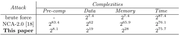
Table 1.Comparison with the best previous attack on the full Grain v1

Attack Complexities

Pre-comp Data Memory Time

brute force - 27.4 ₂7.4 ₂87.4

NCA-2.0 [18] 283.4 262 265.9 276.1

This paper 28.1 219 228 275.7

1

The time complexity unit here is 1 cipher tick as in [18] and the da-ta/memory complexity unit is 1 bit.

and then applied to Grain v1 in Section 5, respectively. In Section 6, practical simulations both on Grain v1 itself and on the reduced version are provided. Finally, some conclusions are drawn and future work is pointed out in Section 7.

2 Description of Grain v1

Grain v1 is a bit-oriented stream cipher, which consists of a pair of linked 80-bit shift registers, one is a linear feedback shift register (LFSR) and anoth-er is a non-linear feedback shift registanoth-er (NFSR), whose states are denoted by (li, li+1, ..., li+79) and (ni, ni+1, ..., ni+79) respectively. The updating function of the LFSR is li+80 =li+62⊕li+51⊕li+38⊕li+23⊕li+13⊕li and the updating

function of the NFSR is

ni+80=li⊕ni+62⊕ni+60⊕ni+52⊕ni+45⊕ni+37⊕ni+33⊕ni+28⊕ni+21

⊕ni+14⊕ni+9⊕ni⊕ni+63ni+60⊕ni+37ni+33⊕ni+15ni+9

⊕ni+60ni+52ni+45⊕ni+33ni+28ni+21⊕ni+63ni+45ni+28ni+9

⊕ni+60ni+52ni+37ni+33⊕ni+63ni+60ni+21ni+15

⊕ni+63ni+60ni+52ni+45ni+37⊕ni+33ni+28ni+21ni+15ni+9

⊕ni+52ni+45ni+37ni+33ni+28ni+21.

The keystream generation phase, shown in Fig.1, works as follows. The

com-NFSR

NFSR _Å_Å_Å LFSRLFSR

( )

h x

Å Å Å

Fig. 1.Keystream generation of Grain v1

(5)

h(x) =x1⊕x4⊕x0x3⊕x2x3⊕x3x4⊕x0x1x2⊕x0x2x3⊕x0x2x4⊕x1x2x4⊕x2x3x4, which is chosen to be balanced and correlation immune of the ﬁrst order with the variablesx0, x1, x2, x3andx4corresponding to the tap positionsli+3,li+25,

li+46,li+64 andni+63 respectively. The outputzi is taken aszi =

⊕

k∈Ani+k⊕

h(li+3, li+25, li+46, li+64, ni+63),where A={1,2,4,10,31,43,56}. The details of the initialization phase are omitted here, the only property relevant to our work is that the initialization phase is invertible.

3 Preliminaries

In this section, some basic deﬁnitions and lemmas are presented with a brief review of the previous near collision attack on Grain v1 in [18]. The following notations are used hereafter.

- wH(·) : the Hamming weight of the input argument.

- d: the Hamming weight of the internal state diﬀerence (ISD). - l: the bit length of the keystream vector.

- n: the bit length of the internal state, whether restricted or not. - ∆x: the value of the ISD, whether restricted or not.

- V(n, d) : the total number of the ISDs withwH(∆x)≤d.

- Ω: the number of CPU-cycles to generate 1 bit keystream in Grain v1 in software.

3.1 Basic Conceptions and Lemmas

Let Bd = {∆x ∈ F2n|wH(∆x) ≤ d} = {∆x1, ∆x2, ..., ∆xV(n,d)} and |Bd| =

V(n, d) =∑d_i₌₀(n_i), where| · |denotes the cardinality of a set. Twon-bit strings

s,s′are said to bed-near-collision, ifwH(s⊕s′)≤dholds. Similar to the birthday

paradox, which states that two random subsets of a space with 2n _{elements are}

expected to intersect when the product of their sizes exceeds 2n_{, we present the}

following generalized lemma, which includes the d-near-collision Lemma in [18] as a special case.

Lemma 1 Given two random setsA andB consisting ofn-bit elements and a condition set D, then there exists a pair (a, b) ∈ A×B satisfying one of the conditions in D if

|A| · |B| ≥c·2

n

|D| (1)

holds, wherecis a constant that determines the existence probability of one good pair (a, b).

Proof. We regard eachai ∈A andbj ∈B as an uniformly distributed random

variable with the realization values in Fn

2. Let A = {a1, a2, ..., a_|A|} and B =

(6)

of the conditions inDbrieﬂy as (ai, bj)∈D. Letϕbe the characteristic function

of the eventϕ((ai, bj)∈D), i.e.,

ϕ((ai, bj)∈D) =

{

1 if (ai, bj)∈D

0 otherwise.

For 1 ≤ i ≤ |A| and 1≤ j ≤ |B|, the number NA,B(D) of good pairs (ai, bj)

satisfying (ai, bj) ∈ D is NA,B(D) =

∑_|A| i=1

∑_|B|

j=1 ϕ((ai, bj) ∈ D). Thus, the expected value ofNA,B(D) of the pairwise independent random variables can be

computed asE(NA,B(D)) =|A| · |B| ·|₂Dn|.Therefore, if we choose the sizes ofA

andB satisfying Eq. (1), the expected number of good pairs is at leastc. ⊓⊔ While when D =Bd, Lemma 1 reduces to the d-near-collision Lemma in [18],

Lemma 1 itself is much more general in the sense that D could be an arbi-trary condition set chosen by the adversary, which provides a lot of freedom for cryptanalysis. Another issue is the choice ofc. In [16], the relation between the choice of the constant c and the existence probability of ad-near-collision pair is illustrated as follows for random samples:

Pr(d-near-collision) =

  

0.606 ifc= 1 0.946 ifc= 3 0.992 ifc= 5.

As stated in [16], these relations are obtained from the random experiments with a modest size, i.e., for each c value, 100 strings of length 40 to 49 for d-values from 10 to 15 are generated,not in a real cipher setting.

Remarks.In a concrete primitive scenario, it is found that the constantc some-times needs to be even larger to assure a high existence probability of near colli-sion good pairs. In our experiments, we ﬁnd that the above relation does not hold for Grain v1 and its reduced versions. In these cases, we have to setc= 8 or even

c= 10 to have an existence probability as high as desirable for the subsequent attack procedures. We believe that for each cipher, the choice of the constantc

and its correspondence to the existence probability of a near collision pair is a fundamental measure related to the security of the primitive. The following fact is used in our new attack.

Corollary 1. For a speciﬁed cipher and a chosen constant c, let A and B be the internal state subsets associated with the observable keystream vectors, where each element ofAandBis ofn-bit length. If we choose|A|= 1and|B| ≥c·_|2_Dn_|, then there exists an elementbi∈Bsuch that the pair(a, bi)with the only element

a∈A forms ad-near collision pair with a probability dependent onc.

(7)

In [18], the two setsAandB are chosen to be of equal size, i.e.,|A|=|B|to minimize the data complexity, in which case the adversary has to deal with all the candidate state positions one-by-one. Instead, Corollary 1 is used in our new attack on Grain v1 via the self-contained method introduced later in Section 4.3, to restore the restricted internal state deﬁned below, at a speciﬁed chosen position along the keystream segment under consideration.

Deﬁnition 1. For a speciﬁed cipher, the subset x= (xi0, xi1, . . . , xin−1)of the

full internal state associated with a given keystream vector z = (zj0, zj1, . . . , zjl−1)is called the restricted internal state associated withz.

We choose the following deﬁnition of the restricted BSW sampling resistance in stream ciphers.

Deﬁnition 2. Let z = (zj0, zj1, . . . , zjl−1) be the known keystream vector

se-lected by the adversary, if l internal state bits in the restricted internal state x associated withzcould be represented explicitly byzand the other bits inx,l is called the restricted BSW sampling resistance corresponding to(x,z).

It is well known that Grain v1 has a sampling resistance of at least 18 [18], thus from Deﬁnition 2, we have l ≤ 18. Actually, we prefer to consider small values oflin our analysis to reduce the memory complexity and to facilitate the veriﬁcation of theoretical predictions. Note that here the indicesj0, j1, . . . , jl−1, either consecutive or inconsecutive, could be chosen arbitrarily by the adver-sary. The restricted BSW sampling inherits the linear enumeration nature of the classical BSW sampling in [4], but unlike the classical BSW sampling, the new sampling does not try to push this enumeration procedure as far as possible, it just enumerates a suitable number of steps and then terminates.

3.2 The Previous Near Collision Attack

At FSE 2013, a near collision attack on Grain v1 was proposed in [18], trying to identify a near collision in the whole internal state at diﬀerent time instants and to restore the two involved states accordingly. For such an inner state pair, the keystream preﬁxes they generate will be similar to each other and the dis-tribution of the KSDs are non-uniform.

(8)

theoretical attack. In [18], the examination of the candidate state pairs is exe-cuted by first recovering the two internal states from the specified ISD. For the LFSR part, this is of no problem since the LFSR updates independently; but for the NFSR part, it is really a problem in [18]. Though the adversary knows the two specified keystream vectors and their corresponding ISD, it is still difficult to restore the full 80-bit NFSR state in such an efficient way that this routine could be invoked a large number of times. Besides, the special table technique assumes that about 50% of all the possible ISDs could be covered on average, which is very hard to verify for the full Grain v1, thus the successful probability of this attack cannot be guaranteed.

In the following, we will show that the adversary need not to recover the full internal state at once when making the examination, actually speciﬁed subsets of the internal state could be restored more eﬃciently than previously thought to be possible, thus the time/memory complexities of the new attack can be consid-erably reduced with an assured success probability andwithout any assumption in the complexity manipulation.

4 Fast Near Collision Attacks

In this section, we will describe the new framework for fast near collision attacks, including both the pre-computation phase and the online attack phase, with the theoretical justiﬁcations.

4.1 General Description of Fast Near Collision Attacks

The new framework is based on the notion of the restricted internal state corre-sponding to a ﬁxed keystream vector, which is presented in Deﬁnition 1 above. Givenz= (zj0, zj1, . . . , zjl−1) withzji (0≤i≤l−1) not necessarily being

con-secutive in the real keystream, the corresponding restricted internal statexforz is determined by the output functionf together with its tap positions, and the state updating function g of the cipher, i.e., induced by the intrinsic structure of the cipher. Besides, from the keystream vectorz, it is natural to look at the augmented function for z.

Definition 3. For a specified cipher with the output function f and the state updating function g, which outputs one keystream bit in one tick, the lth-order augmented functionAf :F|₂x|→Fl₂ for a given(x,z)pair is defined asAf(x) = (f(x), f(gi1_(x))_{, . . . , f}₍_gil−1_(x))).

(9)

Algorithm 1FNCA

Parameters:index: the concrete value of a KSD

prefix: the concrete value of a keystream vector

Oﬄine:foreach combination of (index,prefix)do

Construct the table T[index,prefix], projecting from the KSD indexto all the possible ISDs sorted by the occurring rates

end for

Input: A keystream segmentz_{total = (}zj0, zj1, . . . , zjl−1, zjl, . . . , zjl+γ)

Online: Recover the full internal statex_{full matching with}z_total

1: Dividez_{total into}αoverlapping partszi(1≤i≤α) and a suﬃxzµ

2:fori= 1 toαdo

3: get the candidates listLiof the restricted internal statexiforzi

4:end for

5: MergeLis to get a candidate list for the possible partial statexmerge

6:foreach candidate ofxmerge do

7: restorex_{full and test the consistency with the suﬃx}zµ

The following proposition provides new insights on what inﬂuence the whole internal state size has on the feasibility of a near collision attack.

Proposition 1. For a speciﬁed cipher and two keystream vectorszand z′, the KSD ∆z =z⊕z′ only depends on the ISD ∆x = x⊕x′ and the values of x andx′, whatever the diﬀerence and the values in¯x, the other parts of the whole internal state.

Proof. It suffices to see the algebraic expressions of the keystream bits under consideration. By taking a look at the input variables, we have the claim. ⊓⊔ Offline.Proposition 1 makes the pre-computation phase in FNCA quite differ-ent from and much more efficidiffer-ent than that in the previous NCA in [18]. Now we need not to exhaustively search through all the possible ISDs over the full internal state, which is usually quite large, instead we just search through all the possible ISDs over a specified restricted internal state corresponding to a given keystream vector, which is usually much shorter compared to the full internal state. In Algorithm 1, we use two parametersindexandprefixto characterise this difference withindexbeing the KSD andprefixbeing thevalue of one of the two specified keystream vectors. For each possible combination of (index, prefix), we construct an individual table for the pair. Thus, many relatively small tables are built instead of one large pcomputed table, which greatly re-duces the time/memory complexities of the offline phase, improves the accuracy of the pre-computed information, and finally assures a high success rate of the new attack.

Online.With the differential tables prepared in the offline phase, the adversary first tries to get some candidates of the target restricted internal state x1 and

to ﬁlter out as much as possible wrong candidates of x1 in a reasonable time

complexity. Then he/she moves to another restricted internal statex2, possibly

overlapped with x1, but not coincident with x1, and get some candidates of

(10)

acceptable time/memory complexities and merge the candidate listsLitogether

to get a candidate list of possible partial state x_{merge. Finally, from} x_merge, he/she tries to retrieve the full internal state and check the candidates by using the consistency with the keystream segment.

There are three essential problems that have to be solved in this process. The first one is how to efficiently get the candidates for each restricted internal state and further to filter out those wrong values as much as possible in each case? The second is how to efficiently merge these partial states together without the overflowing of the number of possible internal state candidates, i.e., we need to carefully control the increasing speed of the possible candidates during the merging phase. At last, we need to find some very efficient method to restore the other parts of the full internal state given xmerge, which lies at the core of the routine. We will provide our solutions to these problems in the following sections.

4.2 Oﬄine Phase: Parameterizing the Diﬀerential Tables

Now we explain how to pre-compute the diﬀerential tables T[index,prefix], conditioned on the event that the value of one of the two keystream vectors is

prefix when the KSD is index. Letx = (xi0, xi1, . . . , xin−1) be the restricted

internal state associated with z = (zj0, zj1, . . . , zjl−1), for such a chosen (x,z)

pair, Algorithm 2 fulﬁlls this task. Algorithm 2 is the inner routine of the pre-computation phase of FNCA in the general case, where N1 and N2 are the two random sampling sizes when determining whether a given ISD ∆x of the restricted internal statexcould generate the KSDindexand what the occurring probability is. Algorithm 2 is interesting in its own right, though not adopted in the state recovery attack on Grain v1 in Section 5. It can be applied in the most general case with the theoretical justiﬁcation when dedicated pre-computation is impossible.

Algorithm 2Constructing the diﬀerential table T[index,prefix] 1:foreach ISD∆xs.t.wH(∆x)≤ddo

2: fori= 1toN1 do

3: determine whether∆xcould generate the speciﬁed KSDindex 4: if yesthen

5: forj= 1toN2 do

6: generate randomxs.t.Af(x) =prefixand form the pair (x,x⊕∆x) 7: computez=Af(x) andz′=Af(x⊕∆x)

8: count the number of timescounterthat∆z=z⊕z′=index 9: store the ratiocounter/N2 with∆xin T[index,prefix]

10: Sort the ISDs according to the occurring rates

From V(n, d) = ∑d_i₌₀(n_i), the time complexity of Algorithm 2 is P = 2·

(11)

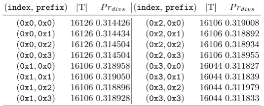
In Table 2, the global information of the 16 T tables for Grain v1 with the 23 original variables whenl= 2 is shown, whereP rdivs is deﬁned as follows.

Table 2.The summary of the pre-computation phase of Grain v1 for 2-bit keystream vector with the 23 original variables

(index,prefix) |T| P rdivs (index,prefix) |T| P rdivs

(0x0,0x0) 16126 0.314426 (0x2,0x0) 16106 0.319008 (0x0,0x1) 16126 0.314434 (0x2,0x1) 16106 0.318892 (0x0,0x2) 16126 0.314504 (0x2,0x2) 16106 0.318934 (0x0,0x3) 16126 0.314504 (0x2,0x3) 16106 0.318955 (0x1,0x0) 16106 0.318958 (0x3,0x0) 16044 0.311827 (0x1,0x1) 16106 0.319050 (0x3,0x1) 16044 0.311839 (0x1,0x2) 16106 0.318896 (0x3,0x2) 16044 0.311979 (0x1,0x3) 16106 0.318928 (0x3,0x3) 16044 0.311833

Definition 4. For each T[index,prefix], let|T|be the number of ISDs in the table, the diversified probability of this table is defined asP rdivs =

∑

∆x∈TPr∆x |T| ,

where∆x ranges over all the possible ISDs in the table.

The diversified probability of a T[index,prefix] table measures the average reducing effect of this table that for a random restricted internal state x such thatAf(x) =prefix, flip the bits inxaccording to a∆x∈T and getx′, then with probabilityP rdivs,Af(x⊕∆x) =prefix⊕index. From Definition 4, the

success rate of the new FNCA is quite high, for we have taken each possible ISD into consideration in the attack.

Corollary 2. From Table 2, if theindexis ﬁxed, then the4P rdivss

correspond-ing to different prefixes are approximately the same, i.e., the 4 T tables have almost the same reducing effect for filtering out wrong candidates.

Corollary 2 is the basis of the merging operation in the online attack phase, which assures that with the restricted BSW sampling resistance of Grain v1 and the self-contained method introduced later, the partial state recovery procedure will not be aﬀected when the keytream vector under consideration has changed its value along the actual keystream. If the keystream vector under consideration has the valueprefix, the adversary uses the valueprefix⊕indexin the computing stage of the self-contained method to have the KSD remaining the same.

4.3 Online Phase: Restoring and Distilling the Candidates

(12)

Algorithm 3The reﬁned self-contained method 1: Initializei= 0

2:while i≤c·_|2_Dn_| do

3: loadxwith a new random value so that it generatesz⊕index 4: foreach possible ISD∆xin T[index,z⊕index]do

5: computex′=x⊕∆x

6: if x′ generatesz then

7: putx′into the candidates listL

8: end if

9: end for

10: i=i+ 1 11:end while

The original self-contained method was proposed in [16], whose idea is to make a tradeoff between the data and the online time complexity in such a way that the second setB of keystream vectors in Lemma 1 is generated by the adversary himself, thus he also knows the actual value of the corresponding internal state that generates the keystream vector. Therefore, given the ISD from the pre-computed tables, the adversary could just xor the ISD with the internal state matching with the keystream vector inB to get the candidate internal state for the keystream vectors in A. In Algorithm 3, it is quite possible that although obtained from a different new starting value for the restricted internal state x, some candidatesx′ will collide with the already existing element in the list, thus the final number of hitting values in the list is not so much as the number of invoking times c· _|2_Dn_|. The following theorem gives the expected value of the actual hitting numbers.

Theorem 1. Let b be the number of all the values that can be hit and a =

c· _|2_Dn_| · |T| ·Pdivs, then after one invoking of Algorithm 3, the mathematical

expectation of the ﬁnal number rof hitting values in the list is

E[r] =

a

∑

r=1

(b r

)

·r!·{a_r}·r

ba , (1)

where{a_r}is the Stirling number of the second kind,(b_r)is the binomial coeﬃcient andr! is the factorial.

Proof. Note that the Stirling number of the second kind [17] {a_r} counts the number of ways to partition a set of a objects into r non-empty subsets, i.e., each way is a partition of theasubjects, which coincides with our circumstance. Thus we can model the process of Algorithm 3 as follows.

We throwaballs intobdiﬀerent boxes, and we want to know the probabil-ity that there are exactly r boxes having some number of balls in. From this converted model, we can see that the size of the total sample space isba_{, while}

(13)

1. Choose r boxes to hold the thrown balls, there are (_rb) ways to fulﬁll this step.

2. permute these rboxes, there arer! ways to fulﬁll this step.

3. partition thea balls intornon-empty sets, this is just the Stirling number of the second kind{a_r}.

Following the multiplication principle in combinatorics, the size of our expected event is just the product of the above three. This completes the proof. ⊓⊔ We have made extensive experiments to verify Theorem 1 and the simulation results match the theoretical predictions quite well. Back to the self-contained method setting,ais just the number of valid candidates satisfying the conditions that the KSD isindexand one of the keystream preﬁx isprefix, of which some may be identical due to the ﬂipping according to the ISDs in T.

In general, the opponent can build a table for the functionf, mapping the partial sub-states to the keystream vectorz, to get a full list of inputs that map to a givenz. In order to reduce the candidate list size in a search, he may somehow choose a smaller list of inputs that map to z, and hope that the correct partial state is still in the list with some probability p, depending on the size of the list. The aim of the distilling phase is to exploit the birthday paradox regarding d-near collisions, local diﬀerential properties off, and the self-contained method to derive smaller lists of input sub-states so that the probability that the correct state is in the list is at leastp. From Lemma 1, with a properly chosen constant

c, the correct internal statexwill be in the listLwith a high probability, e.g., 0.8 or 0.95. For a chosen (x,z) pair, the candidates reduction process is depicted in Algorithm 4.

Algorithm 4Distilling the candidates

Parameter: a well chosen constantβ 1:fori= 1 toβ do

2: run Algorithm 3 to get the candidates listLi

3:end for

4: Initialize a listU and letU =L1

5:fori= 2 toβ do

6: intersectU withLi, i.e.,U ←U∩Li

The next theorem characterizes the number of candidates passing through the distilling process in Algorithm 4.

Theorem 2. The expected number of candidates in the list U in Algorithm 4 after β −1 steps of intersection is |U1| ·(E_b[r])β−1, where |U1| = |L1| is the number of candidates present in the ﬁrst listL1 andE[r]is the expected number of hitting values in one single invoking of Algorithm 3.

Proof. For simplicity, let |Ui|=fi denote the cardinality of the candidates list

after i−1 steps of intersection for 1≤i≤β−1. Note that in the intersection process, if there are fi candidates in the current listU, then at the next

(14)

Letfi → fi+1 denote the event that there arefi+1 elements left after one intersection operation on thefi elements in the currentU. The expected value

offi+1isE[fi+1] =

∑fi j=0

(fi j

)

·(E_b[r])j·(1−E_b[r])fi−j·_j₌_f

i·E_b[r].Thus we have

the following recursion

fβ−1=fβ−t−1·

t

∏

i=1 (E[r]

b ) =|U1|·( E[r]

b )·( E[r]

b )· · · · ·( E[r]

b )

| {z }

β−1

=|U1|·(

E[r]

b )

β−1_,

which completes the proof. ⊓⊔

Algorithm 5Improving the existence probability of the correctx Parameter: a well chosen constantγ

1:fori= 1 toγ do

2: run Algorithm 4 to get the candidates listUi

3:end for

4: Initialize a listV and letV =U1

5:fori= 2 toγ do

6: unionV withUi, i.e.,V ←V∪Ui

Theorem 2 partially characterizes the distilling process in theory. Now the crucial problem is what thereduction effectof this process is, which is determined by the choice of the constantc intrinsic to each primitive and the number of variables involved in the current augmented function. From the cryptanalyst’s point of view, the larger β is, the lower the probability that the correctxis involved in each generated list, thus it is better for the adversary to make some tradeoff betweenβ and this existence probability. Algorithm 5 provides a way to exploit this tradeoff to get some higher existence probability of the correct restricted internal statex.

In Algorithm 5, several candidate lists are ﬁrst generated by Algorithm 4 with a number of intersection operations for each list, then these lists are uniﬁed together to form a larger list so that the existence probability of the correct x becomes higher compared to that of each component list.

Theorem 3. Let the expected number of candidates in list V in Algorithm 5 after i(1≤i≤γ)steps of union be Fi, then the following relation holds

Fi+1=Fi+|Ui+1| −

|U∑i+1|

j=0

(Fi j

)

·(Fi+1−Fi |Ui+1|−j

) (Fi+1

|Ui+1|

) ·j , 1≤i≤γ−1 (2)

where|F1|=|U1|.

Proof. Note that when a newUi+1is uniﬁed intoV, we haveFi+1=Fi+|Ui+1|−

(15)

Theorem 3 provides a theoretical estimate of |V|, which is quite close to the experimental results. After gettingV forx1, we move to the next restricted in-ternal statex2, as depicted in Algorithm 1 until we recovered all theαrestricted internal states. Then we merge the restored partial states xi for 1 ≤i ≤α to

cover a larger part of the full internal state. We have to recover the full internal state conditioned on xmerge. The next theorem describes the reduction eﬀect when merging the candidate lists of two restricted internal states.

Theorem 4. Let the candidates list for xi be Vi, then when merging the

can-didates list Vi for xi and Vi+1 for xi+1 to cover an union state xi∪xi+1, the expected number of candidates for the union state xi∪xi+1 is

E[|Vxi∪xi+1|] =

|Vi| · |Vi+1|

|Vi∩Vi+1|

,

whereVxi∪xi+1 is the candidates list for the union statexi∪xi+1.

Proof. Denote the bits inxi∩xi+1 byI=I0, I1,· · ·, I_|xi∩xi+1|−1 when merging

the two adjacent restricted internal states xi and xi+1, then we can groupVi

and Vi+1 according to the|xi∩xi+1| concrete values of I. For the same value pattern of the common bits inI, we can just merge the two states xi and xi+1 by concatenating the corresponding candidate states together directly. Thus, the expected number of candidates for the union state is

E[|Vxi∪xi+1|] =

|Vi|

|Vi∩Vi+1|·

|Vi+1|

|Vi∩Vi+1| · |

Vi∩Vi+1|=|

Vi| · |Vi+1|

|Vi∩Vi+1|

,

which completes the proof. ⊓⊔

Corollary 3. In the merging process of Algorithm 1, let MA and MB be two

partial internal states, each merged from possibly several restricted internal states respectively, then when merging MA and MB together, the expected number of

candidates for the union stateMA∪MB isE[|MA∪MB|] = |_|M_MA|·|MB| A∩MB|.

Proof. It suﬃces to note the statistical independence of each invoking of

Algo-rithm 5 and Theorem 4. ⊓⊔

Finally, we present the theorem on the success probability of Algorithm 5. Theorem 5. Let the probability that the correct value of the restricted internal statexwill exist inV be Prx, then we have Prx= 1−(1−(Pc)β)γ, wherePc is

the probability that the correct value of the restricted internal state xexist inU

for one single invoking of Algorithm 3.

Proof. From Algorithm 4 and 5, the probability that for all theγ Uis, the correct

value ofxdoes not exist in the list is (1−(Pc)β)γ, thus the opposite event has

(16)

5 State Recovery Attack on Grain v1

Now we demonstrate a state recovery attack on the full Grain v1. The new attack is based on the FNCA framework described in Section 4 with some techniques to control the attack complexities.

5.1 Rewriting Variables and Parameter Conﬁguration

From the keystream generation of Grain v1, we havezi=

⊕

k_∈Ani+k⊕h(li+3,

li+25, li+46, li+64, ni+63), where A = {1,2,4,10,31,43,56}, i.e., one keystream bitzi is dependent on 12 binary variables, of which 7 bits from the NFSR form

the linear masking bit ⊕_k_∈Ani+k, 4 bits from the LFSR and ni+63 from the NFSR are involved in the ﬁlter functionh.

For a straightforward FNCA on Grain v1, even considering two consecutive keystream bits, we have to deal with 23 binary variables simultaneously at the beginning of the attack. Thus the number of involved variables will grow rapidly with the running of the attack, and probably overﬂow at some intermediate point. To overcome this diﬃculty, we introduce the following two techniques to reduce the number of free variables involved in the keystream vectors.

Letxi=ni+1⊕ni+2⊕ni+4⊕ni+10⊕ni+31⊕ni+43⊕ni+56, then we have

zi=xi⊕h(li+3, li+25, li+46, li+64, ni+63). (3) There are only 6 binary variables xi, li+3, li+25, li+46, li+64, ni+63 involved in Eq.(3) and if we consider a keystream vector z = (zi, zi+1), there are only 12 variables now, almost reduced by half compared to the previous number 23. Note that the rewriting technique is known to be useful in [9] before in algebraic attacks on stream ciphers.

Besides, we can still use the linear enumeration procedure as in the BSW sampling case to reduce the variables further. Precisely, from Eq.(3), we have

xi = zi⊕h(li+3, li+25, li+46, li+64, ni+63), thus for the above keystream vector z= (zi, zi+1), we could actually deal with 10 binary variables only, making xi

andxi+1 dependent on the other 10 variables and (zi, zi+1). Algorithm 6The pre-computation after rewriting variables

Parameter: matrixP1 of size 2l×V(n, d) withP1[i][j]̸= 0 if the ISD

jcould generate the KSDiand 0 otherwise 1: Initialize the table T[index,prefix]

2:foreach possible value ofx do

3: foreach ISD∆xs.t.wH(∆x)≤ddo

4: determine whetherfsr(x) =prefixandfsr(x⊕∆x) =prefix⊕index

5: if yesthenP1[index][∆x] =P1[index][∆x] + 1

6:foreach ISD∆xs.t.wH(∆x)≤ddo

7: setP1[index][∆x]/|x|as the occurring rate of∆x

8: Sort the ISDs according to the occurring rates

(17)

T[index,prefix] for the chosen attack parameters shown in Algorithm 6, which results in the accurately computed occurring probabilities compared to Algo-rithm 2 in Section 4.2, where fsr(·) is the evaluation of the underlying stream

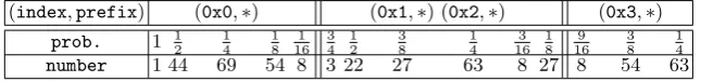
cipher. The complete pre-computation table of Grain v1 is listed in Table 3 for Table 3. The full Pre-computation information of Grain v1 after rewriting variables whend= 3

(index,prefix) (0x0,∗) (0x1,∗) (0x2,∗) (0x3,∗) prob. 1 1₂ 1₄ 1₈ ₁₆1 3₄ 1₂ 3₈ 1₄ ₁₆3 1₈ ₁₆9 3₈ 1₄

number 1 44 69 54 8 3 22 27 63 8 27 8 54 63

d= 3, where∗ indicates that theprefix could take any value from0x0to0x3

due to the same distribution for diﬀerent preﬁx values andnumber denotes the number of ISDs having the corresponding occurring probability.

From Table 3 and Definition 4, we have the following corollary on the diver-sified probabilities of different pre-computed tables.

Corollary 4. For the pre-computation table of Grain v1 after rewriting vari-ables, we have

Prdivs=

      

0.269886, if index=0x0

0.293333, if index=0x1

0.293333, if index=0x2

0.324000, if index=0x3.

Proof. From Deﬁnition 4, we haveP rdivs = ∑

∆x∈TPr∆x

|T| , it suﬃces to substitute

the variables with the values from Table 3 to get the results. ⊓⊔ From Corollary 4, we choose the KSD to be0x0in our attack, for in this case the reduction eﬀect is maximized with the minimum Prdivs. Under this condition, we

have run extensive experiments to determine the constantcfor Grain v1, which is shown in the following table, wherePcis the probability that the correct value of

the restricted internal state exists in the resultant list after one single invoking of Algorithm 3. Based on Table 4, we have run a number of numerical experiments Table 4.The correspondence between the constantcand the existence probability for index= 0x0

c 5 6 7 8 9 10

Pc0.757137 0.816551 0.860638 0.89502 0.92114 0.94644

c 11 12 13 14 15 16 Pc 0.95423 0.96573 0.97567 0.98021 0.985524 0.989411

to determine the appropriate conﬁguration of attack parameters and found that

c= 10 provides a balanced tradeoﬀ between various complexities.

(18)

augmented functionAf), we ﬁnd that if β= 21 andγ= 6, then we get Prxi =

1−(1−0.9464421₎6 _{= 0}_._{896456 from Theorem 5. We have tested this fact in} experiments for 106_{times, and found that the}_average _{value of the success rate} well matches to the theoretical prediction. Besides, we have also found that under this parameter conﬁguration, the number of candidates in the listV for the current restricted internal statexis 848≈29.73_{, which is also quite close to} the theoretical value 29.732 _{got from Theorem 3.}

Corollary 5. For Grain v1 when c = 10and l = 2, the conﬁguration that the resultant candidate list V is of size848 with the average probability of0.896456 for the correct restricted internal state being in V is non-random.

Proof. Note that in the pure random case, the list V should have a size of 210_·₀_._{896456 = 917}_._{971 with the probability 0}_._{896456; now in Grain v1, we get} a list V of size 848 with the same probability. In the pure random case, we have

E[|V|] =µ= 210·0.896456 = 917.971, σ=

√

210·1 4 ·

3

4 = 13.8564. Further, µ−_σ848 =917₁₃.971_.₈₅₆₄−848 = 5.0497; from Chebyshev’s inequality, the conﬁg-uration (848,0.896456) is far from random with the probability around 0.99. ⊓⊔ Now we are ready to describe the attack in details based on the above attack parameter conﬁguration.

5.2 Concrete Attack: Strategy and Proﬁle

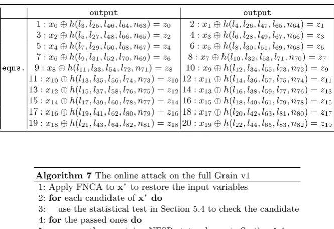
First note that if we just run Algorithm 1 along a randomly known keystream segment to retrieve the overlapping restricted internal states one-by-one without considering the concrete internal structure of Grain v1, then we will probably meet the complexity overﬂow problem in the process when the restored internal statexmerge does not cover a large enough internal state, and at the same time, the number of candidates and the complexity needed to check these candidates will exceed the security bound already. Instead, we proceed as follows to have a more eﬃcient attack. First observe that if we target the keystream vector z = (zi, zi+1) through rewriting variables in Table 5 and restore the variables therein by our method, then for such a 2-bit keystream vector, we can obtain 8 LFSR variables involved in thehfunction and 2 NFSR bitsni+63, ni+64, together with 2 linear equationsxi=

⊕

k_∈Ani+k andxi+1=

⊕

k_∈Ani+k+1on the NFSR variables. If we repeat this procedure for the time instants from 0 to 19, then from

zi =xi⊕h(li+3, li+25, li+46, li+64, ni+63), we will have li+3+j, li+25+j, li+46+j,

li+64+j andni+63+j for 0≤j ≤19 involved in Table 5.

(19)

Table 5.The target keystream equations ﬁrst exploited in our attack

output output

1 :x0⊕h(l3, l25, l46, l64, n63) =z0 2 :x1⊕h(l4, l26, l47, l65, n64) =z1

eqns. 9 :x8⊕h(l11, l33, l54, l72, n71) =z8 10 :x9⊕h(l12, l34, l55, l73, n72) =z9

Algorithm 7The online attack on the full Grain v1 1: Apply FNCA tox∗to restore the input variables 2:foreach candidate ofx∗do

3: use the statistical test in Section 5.4 to check the candidate 4:forthe passed onesdo

5: recover the remaining NFSR state, shown in Section 5.4 6:foreach candidate ofx_fulldo

7: check the consistency with the available keystream

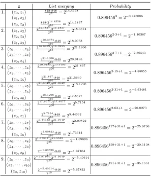
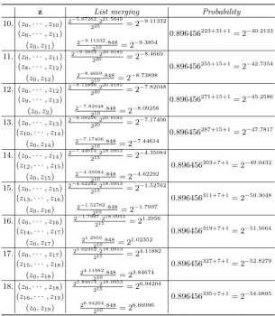
After knowing the LFSR part and more than half of the NFSR, we could ﬁrst identify the correct LFSR state by the Walsh distinguisher, then the remaining NFSR state could easily be retrieved with an algebraic attack, both shown in the following Section 5.4. Note that in Table 6 and 7, the list size for each merging operation is listed in the middle column, based on Theorem 4 and Corollary 3. For example, let us look at the 1st step. The reason that 25 _{is used instead} of 26 _{in denominator is that the} _x

i variables are not freely generated random

variables, for we have made them linearly dependent on the 5 variables in h

function and the corresponding keystream bits to fulﬁll our criterion on the pre-computed tables. 214.4558 _{is the list size when merging the two restricted} internal states corresponding to (z0, z1) and (z1, z2), respectively. After merg-ing (z0, z1) and (z1, z2), we get a list for the restricted internal state of the 3-bit keystream vector (z0, z1, z2). Now we further invoke the self-contained method for the keystream vector (z0, z2), which consists of onlyz0and the non-consecutive

(20)

Table 6.The attack process for recoveringx∗(1)

z List merging Probability

1. (z0, z1) 848₂·5848 = 2

14.4558

(z1, z2) 0.8964563= 2−0.473086

(z0, z2) 848·2

14.4558

210 = 2

14.1837

2. (z1, z2) 2

14.1837_·₂14.1837

210 = 2

18.3674

(z2, z3) 0.8964562·3+1= 2−1.10387

(z1, z3) 2

18.3674_·₈₄₈

210 = 2

18.0953

3. (z0,· · ·, z3) 2

18.0953_·₂18.0953

215 = 2

21.1906

(z1,· · ·, z4) 0.8964562·7+1= 2−2.36543

(z0, z4) 2

21.1906_·₈₄₈

210 = 2

20.9185

4. (z0,· · ·, z4) 2

20.9185_·₂20.9185

220 = 2

21.837

(z1,· · ·, z5) 0.8964562·15+1= 2−4.88855

(z0, z5) 2

21.837_·₈₄₈

210 = 2

21.5649

5. (z0,· · ·, z5) 2

21.5649_·₂21.5649

225 = 2

18.1298

(z1,· · ·, z6) 0.8964562·31+1= 2−9.93481

(z0, z6) 2

18.1298_·₈₄₈

210 = 2

17.8577

6. (z0,· · ·, z6) 2

17.8577_·₂17.8577

230 = 2

5.7154

(z1,· · ·, z7) 0.8964562·63+1= 2−20.0273

(z0, z7) 2

5.7154_·₈₄₈

210 = 2

5.44332

7. (z0,· · ·, z7) 2

5.44332_·₂21.5649

225 = 2

2.00822

(z3,· · ·, z8) 0.896456127+31+1= 2−25.0736

(z0, z8) 2

2.00822_·₈₄₈

210 = 2

1.73614

8. (z0,· · ·, z8) 2

1.73614_·₂21.5649

225 = 2−

1.69896

(z4,· · ·, z9) 0.896456159+31+1= 2−30.1198

(z0, z9) 2

−1.69896_·₈₄₈

210 = 2−

1.97104

9. (z0,· · ·, z9) 2

−1.97104_·₂21.5649

225 = 2−

5.40614

(z5,· · ·, z10) 0.896456191+31+1= 2−35.1661

(z0, z10) 2

−5.40614_·₈₄₈

210 = 2−

(21)

Table 7.The attack process for recoveringx∗(2)

z List merging Probability

10. (z0,· · ·, z10) 2

−5.67262_·₂21.5649

225 = 2−

9.11332

(z6,· · ·, z11) 0.896456223+31+1= 2−40.2123

(z0, z11) 2

−9.11332_·₈₄₈

210 = 2−

9.3854

11. (z0,· · ·, z11) 2

−9.3854_·₂20.9185

220 = 2−

8.4669

(z8,· · ·, z12) 0.896456255+15+1= 2−42.7354

(z0, z12) 2

−8.4669_·₈₄₈

210 = 2−

8.73898

12. (z0,· · ·, z12) 2

−8.73898_·₂20.9185

220 = 2−

7.82048

(z9,· · ·, z13) 0.896456271+15+1= 2−45.2586

(z0, z2) 2

−7.82048_·₈₄₈

210 = 2−

8.09256

13. (z0,· · ·, z13) 2

−8.09256_·₂20.9185

220 = 2−

7.17406

(z10,· · ·, z14) 0.896456287+15+1= 2−47.7817

(z0, z14) 2

−7.17406_·₈₄₈

210 = 2−

7.44614

14. (z0,· · ·, z14) 2

−7.44614_·₂18.0953

215 = 2−

4.35084

(z12,· · ·, z15) 0.896456303+7+1= 2−49.0432

(z0, z15) 2

−4.35084_·₈₄₈

210 = 2−

4.62292

15. (z0,· · ·, z15) 2

−4.62292_·₂18.0953

215 = 2−

1.52762

(z13,· · ·, z16) 0.896456311+7+1= 2−50.3048

(z0, z16) 2

−1.52762_·₈₄₈

210 = 2−

1.7997

16. (z0,· · ·, z16) 2

−1.7997_·₂18.0953

215 = 2

1.2956

(z14,· · ·, z17) 0.896456319+7+1= 2−51.5664

(z0, z17) 2

1.2956_·₈₄₈

210 = 2

1.02352

17. (z0,· · ·, z17) 2

1.02352_·₂18.0953

215 = 2

4.11882

(z15,· · ·, z18) 0.896456327+7+1= 2−52.8279

(z0, z18) 2

4.11882_·₈₄₈

210 = 2

3.84674

18. (z0,· · ·, z18) 2

3.84674_·₂18.0953

215 = 2

6.94204

(z16,· · ·, z19) 0.896456335+7+1= 2−54.0895

(z0, z19) 2

6.94204_·₈₄₈

210 = 2

(22)

the corresponding internal state subsets, not including the linearly dependent variables. This process is repeated until merging the 20th equation in Table 5.

5.3 Restoring the Internal State of the LFSR

From Table 5,x∗ involves 78 LFSR bits in total, it seems that we need to guess 2 more LFSR bits to have a linear system covering the 80 initial LFSR variables. To have an eﬃcient attack, ﬁrst note that bothl64 andl65 are used 2 times in these equations, thus the candidate values should be consistent on l64 and l65, which will provide a reduction factor of ₂12 =

1

4on the total number of candidates. Further, froml83=l65⊕l54⊕l41⊕l26⊕l16⊕l3, we have a third linear consistency check on the candidates. Hence, the number of candidates after going through Table 6 and 7 is ₂−54.08951 ·2

6.66996_·₂₋3_{= 2}57.7595_{. By guessing 2 more bits}_l 0, l1, we can getl23, l24from the recursionl80+j=l62+j⊕l51+j⊕l38+j⊕l23+j⊕l13+j⊕lj

forj = 0,1. In addition, we can derivel2froml82=l64⊕l53⊕l40⊕l25⊕l15⊕l2. Note that the LFSR updates independently in the keystream generation phase and we also know the positions of the restored LFSR bits either from FNCA or from guessing, thus we could make a pre-computation to store the inverse of the corresponding linear systems with an oﬀ-line complexity of 80_Ω2.8 cipher ticks and a online complexity of 80_Ω2 to ﬁnd the corresponding unique solu-tion, where 2.8 is the exponent for Gauss reduction. This complexity is negligible compared to those of the other procedures. The total number of candidates for the LFSR part and the accompanying partial NFSR state, 22·257.7595= 259.7595, will dominate the complexity.

Remarks. Note that the gain in our attack mainly comes from the following two aspects. First, we exploit the ﬁrst 20-bit keystream information in this pro-cedure in aprobabilistic way, not in a deterministic way, which is depicted later in Theorem 7. Now we target 78 + 20 + 20 = 118 variables, not 160 variables, in a tradeoﬀ-like manner. Here only 98 variables can be freely chosen. This cannot be interpreted in a straightforward information-theoretical way, which is usually evaluated in a deterministic way. Second, we use the pre-computed tables which also contain quite some information on the internal structure of Grain v1 in an implicit way in the attack.

5.4 Restoring the Internal State of the NFSR

(23)

From the above step, the FNCA method has provided the adversary with the NFSR bitsn63+i andxi =ni+1⊕ni+2⊕ni+4⊕ni+10⊕ni+31⊕ni+43⊕ni+56 for 0≤i≤19, i.e., now there are 20 + 20 = 40-bit information available on the NFSR initial state. We proceed as follows to get more information.

Collecting More Linear Equations on NFSR.First note that if we go back 1 step, we getx₋1=n0⊕n1⊕n3⊕n9⊕n30⊕n42⊕n55, i.e., we get 1 more linear equation for free. If we go back further, we could get a series of variables that can be expressed as the linear combination of the known values and the target initial NFSR state variables. On the other side, if we go forwards and take a look at the coeﬃcient polynomial ofx4 in thehfunction, i.e., 1⊕x3⊕x0x2⊕x1x2⊕x2x3, we ﬁnd it is a balanced Boolean function. Thus, the n82+i variables have a

probability of 0.5 to vanish in the resultant keystream bit and the adversary could directly collect a linear equation through the correspondingx20+i variable

at the beginning time instants from 20.

To get more linear equations on the NFSR initial state, we can use the following Z-technique, which is based on the index diﬀerence of the involving variables in the keystream bit. Precisely, if n82+i appears at thez19+i position,

let us look at the end of the keystream equationz26+ito see whethern82+iexists

there or not. If it is not there, then this will probably give us one more linear equation on the NFSR initial variables due to the index diﬀerence 56−43 = 13 >7; if it is there, we could just xor the two keystream equations to cancel out the n82+i variable to get a linear equation on the NFSR initial variables.

Then increaseiby 1 and repeat the above process for the newi. Since the trace of the equations looks like the capital letter ’Z’, we call this technique Z-technique. An illustrative example is provided in Appendix A.

It can be proved by induction that the Z-technique can also be used to express the newly generated NFSR variables as linear combinations of the keystream bits and of the initial state variables in forward direction. In backward direction, it is trivial to do the same task. We have run extensive experiments to see the average number of linear equations that the adversary could collect using the Z-technique, it turns out that the average number is 8, i.e., we could reduce the number of unknown variables in the initial NFSR state to around 80−40−(8− 3) = 35, which facilitates the following linear distinguisher.

The Walsh Distinguisher. First note that the NFSR updating function in Grain v1 has a linear approximation with bias ₅₁₂41, shown below.

n80+i=n62+i⊕n60+i⊕n52+i⊕n45+i⊕n37+i⊕n28+i⊕n21+i⊕n14+i⊕ni⊕e,

where e is the binary noise variable satisfying Pr(e = 0) = 1 2 +

(24)

following form         

c0₀ni0⊕c

0

1ni1⊕ · · · ⊕c

0

34ni34 =kz0⊕e0 c1₀ni0⊕c

1

1ni1⊕ · · · ⊕c

1

34ni34 =kz1⊕e1

..

. ... ...

cδ₀−1ni0⊕c δ₋1

1 ni1⊕ · · · ⊕c δ₋1

34 ni34 =kzδ−1⊕eδ−1,

(3)

whereci

j ∈F2for 0≤i≤δ−1 and 0≤j ≤34 is the coeﬃcient of the remaining NFSR variablenij (0 ≤j ≤34),kzi (0≤i≤δ−1) is the accumulated linear

combination of the keystream bits and the known information from the LFSR part and the partial NFSR state derived before and ei (0 ≤i ≤ δ−1) is the

binary noise variable with the distribution Pr(ei= 0) = 1₂+₅₁₂41.

To further reduce the number of unknown NFSR variables, we construct the parity checks of weight 2 from the above system as follows. First note that the bias of the parity checks is 2·(₅₁₂41)2_{= 2}−6.2849_{from the Piling-up lemma in [14].} Second, this problem is equivalent to the LF2 reduction in LPN solving problems [12], which can be solved in a sort-and-merge manner with a complexity of at mostδ using pre-computed small tables. We have tuned the attack parameters in this procedure and found that ifδ= 219_and_y_{= 15, we could collect}(219−15

2

)

·

215_{= 2}21.9069 _{parity-checks on 35}₋_y_{= 20 NFSR variables of the bias 2}−6.2849_. Note that we could further cancel out 4 more NFSR variables in these parity-checks by only selecting those equations that the corresponding coeﬃcient of the assigned variable is 0, in this way we could easily get 221.9069₂4 = 217.9069

parity-checks on 20−4 = 16 NFSR variables. On the other side, from the unique solution distance in correlation attacks [6, 13], we have

8·16·ln2 1−h(p) = 2

17.5121_<₂17.9069_,

where p= 1₂+ 2−6.2849 and h(p) =−p·logp−(1−p)·log(1−p) is the binary entropy function. Thus, we can have the success probability very close to 1 given 217.9069 _{parity-checks to identify the correct value of the 16 NFSR variables} under consideration. That is, we reach the following theorem.

Theorem 6. If both the LFSR candidate and the partial NFSR state are correct, we can distinguish the correct value of the remaining 16 NFSR variables from the wrong ones with a success probability very close to 1.

Proof. It suﬃces to note that if either the LFSR or the partial NFSR state is wrong, there exists no bias in the system (3), thus following the classical reasoning from correlation attacks in [6, 13], we have the claim. ⊓⊔ Precisely, for each parity-check of weight 2 for the system (3), we have

(cj1

0 ⊕c

j2

0 )ni0⊕(c j1

1 ⊕c

j2

1)ni1⊕ · · · ⊕(c j1

34−y⊕c j2

34−y)ni0 =

2

⊕

t=1

kzjt⊕

2

⊕

t=1