BENGERI, SUDHINDRA S. Differentiated Services Support for the Helios Optical Access Network Testbed. (Under the direction of Dr. George Rouskas.)
BIOGRAPHY
ACKNOWLEDGEMENTS
I would like to thank my parents for everything that they have done for my upbringing and encouraging me to pursue higher education. My fianc´ee, Shilpa, has been a constant source of motivation from the time I took GRE, through the application process and during my masters. I thank her for having stood by me in every decision I have made.
I would like to thank Dr. George N. Rouskas for having given me the opportunity for con-ducting research in the interesting field of WDM access networks, under his able guidance. This thesis would not have be possible without his continual support and advice.
I would like to thank Dr. Harry Perros and Dr. Robert Fornaro for serving on my thesis committee. I would also like to thank Dr. Carla Savage for her suggestions for efficient implementation of the Open-Shopscheduling algorithm.
Contents
List of Figures vii
List of Tables ix
1 Introduction 1
1.1 Broadcast-and-Select Single-Hop WDM Optical Networks . . . 1
1.2 Differentiated Services . . . 2
1.3 Motivation . . . 3
1.4 Thesis Organization . . . 3
2 Background and Related Work 5 2.1 Algorithm design parameters . . . 5
2.2 Scheduling Algorithms . . . 9
2.2.1 Bandwidth Guarantee . . . 11
2.2.2 Delay Guarantee . . . 14
3 System Model and Problem Statement 23 3.1 Network Model . . . 23
3.2 Problem Statement . . . 26
4 Scheduling Algorithms 28 4.1 Preemptive Open-Shop scheduling algorithm . . . 29
4.2 Best-effort traffic allocation for OS . . . 33
4.3 Non-preemptive Open-Shop with tuning latencies . . . 35
4.4 Best-effort traffic allocation for OSTL . . . 38
4.5 Simulation Study . . . 41
5 Optimization Heuristics 50 5.1 Channel Decomposition . . . 51
6 Simulator Implementation 53 6.1 Introduction tons-2 . . . 53
6.2 Nortel’s Diffserv implementation inns-2 . . . 54
7 Numerical Results 71
8 Summary and Future Research 84
8.1 Summary . . . 84 8.2 Future Research . . . 84
List of Figures
3.1 A Broadcast-and-select WDM network . . . 24
4.1 Bipartite graph as constructed by the preemptive open-shop algorithm . . . 32 4.2 Preemptive open-shop schedule without best effort traffic, forN = 5 andC= 3 32 4.3 Algorithm: Best-effort allocation for preemptive open-shop algorithm (BE-OS) 33 4.4 Preemptive open-shop schedule with best effort traffic, forN = 5 andC = 3 35 4.5 Nonpreemptive OSTL schedule without best effort traffic, for N = 5, C = 3
and ∆ = 2 . . . 37 4.6 Nonpreemptive OSTL schedule with best effort traffic, forN = 5,C = 3 and
∆ = 2 . . . 40 4.7 Nonpreemptive OSTL schedule with best effort traffic allocation by BE-OS,
forN = 5,C = 3 and ∆ = 2 . . . 40 4.8 Algorithm: Best effort allocation for the nonpreemptive OSTL algorithm
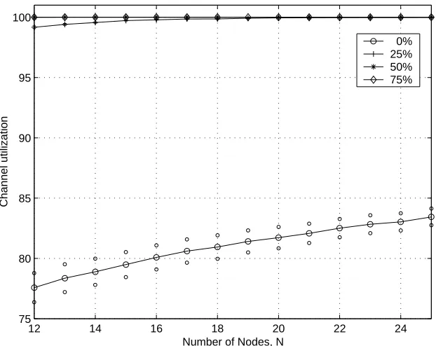
(BE-OSTL) . . . 45 4.9 Channel throughput with BEOS best effort allocation, for C=6 (values
plot-ted with 95% confidence interval) . . . 46 4.10 Channel throughput with BEOS best effort allocation, for C=24 (values
plot-ted with 95% confidence interval) . . . 46 4.11 Channel throughput with BEOSTL best effort allocation, for C=6 (values
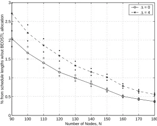
plotted with 95% confidence interval) . . . 47 4.12 Percentage increase in schedule length after BEOSTL best effort allocation,
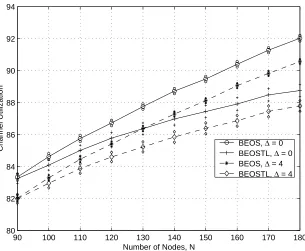
for C=6 (values plotted with 95% confidence interval) . . . 47 4.13 Channel throughput with BEOSTL best effort allocation, for C=24 (values
plotted with 95% confidence interval) . . . 48 4.14 Percentage increase in schedule length after BEOSTL best effort allocation,
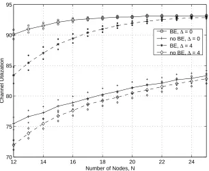
for C=24 (values plotted with 95% confidence interval) . . . 48 4.15 Channel throughput comparisions with OSTL scheduling algorithm, for C=24
(values plotted with 95% confidence interval) . . . 49 4.16 Schedule length comparisions with OSTL scheduling algorithm, for C=24
(values plotted with 95% confidence interval) . . . 49
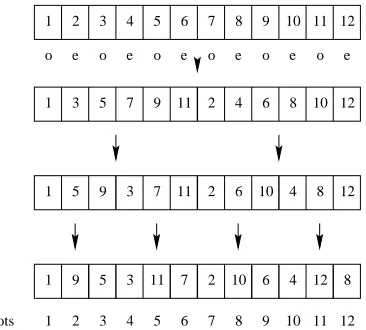
5.3 Decomposition of a 12-slot schedule . . . 52
6.1 Simulation architecture . . . 57
6.2 Components of a Unidirectional Link in ns-2 . . . 59
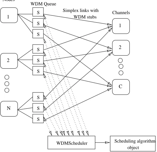
6.3 Class hierarchy of a WDM Queue . . . 61
6.4 Class hierarchy of the optimal scheduler . . . 64
7.1 Average scheduling delay comparision for non-backlogged and backlogged traffic on a 1 Gbps channel with 200 nodes, for a reservation of 40% . . . . 74
7.2 Delay Jitter comparision for non-backlogged and backlogged traffic on a 1 Gbps channel with 200 nodes, for a reservation of 40% . . . 74
7.3 Standard deviation in scheduling delay for non-backlogged and backlogged traffic on a 1 Gbps channel with 200 nodes, for a reservation of 40% . . . . 75
7.4 Average scheduling delay comparision for committed burst size of 6, 12 pack-ets on a 1 Gbps channel with 200 nodes, for 10%−40% reservation . . . 76
7.5 Delay Jitter comparision for committed burst size of 6, 12 packets on a 1 Gbps channel with 200 nodes, for 10%−40% reservation . . . 77
7.6 Standard deviation in scheduling delayfor committed burst size of 6, 12 pack-ets on a 1 Gbps channel with 200 nodes, for 10%−40% reservation . . . 77
7.7 Average scheduling delay comparision with and without channel decomposi-tion on a 1 Gbps channel with 200 nodes, for a reservadecomposi-tion of 40% . . . 78
7.8 Delay Jitter comparision with and without channel decomposition on a 1 Gbps channel with 200 nodes, for a reservation of 40% . . . 79
7.9 Standard deviation in scheduling delay with and without channel decompo-sition on a 1 Gbps channel with 200 nodes, for a reservation of 40% . . . . 79
7.10 Average scheduling delay comparision with and without channel decompo-sition on a 1 Gbps channel with 200 nodes, for committed burst size of 12 packets . . . 80
7.11 Delay Jitter comparision with and without channel decomposition on a 1 Gbps channel with 200 nodes, for committed burst size of 12 packets . . . . 81
7.12 Standard deviation in scheduling delay with and without channel decompo-sition on a 1 Gbps channel with 200 nodes, for committed burst size of 12 packets . . . 81
7.13 Average scheduling delay comparision with and without channel decomposi-tion on a 10 Gbps channel with 200 nodes, for committed burst size of 12 packets . . . 82
7.14 Delay Jitter comparision with and without channel decomposition on a 10 Gbps channel with 200 nodes, for committed burst size of 12 packets . . . . 83
List of Tables
2.1 Classification of algorithms providing bandwidth guarantee. . . 10
2.2 Classification of algorithms providing timing guarantee. . . 10
4.1 Collapsed demand matrix for three processors and five jobs . . . 31
4.2 Combined traffic matrix, with best effort slots allocated by BE-OS . . . 35
7.1 Reservations per node per cycle and resulting schedule lengths . . . 72
Chapter 1
Introduction
1.1
Broadcast-and-Select Single-Hop WDM Optical Networks
Technological advances have dramatically increased electronic processing speeds, however so has the transmission capacity of optical systems. Inevitably, network capac-ity will always be limited by the electronic bottleneck. Wavelength division multiplexing (WDM) eases this opto-electronic speed mismatch by partitioning the enormous optical bandwidth into multiple channels. Each channel carries traffic at data-rate of the interface electronics, possibly at peak electronic speed. By allowing multiple WDM channels to co-exist on a single fiber, one can tap into the huge fiber bandwidth, with the corresponding challenge being design and development of appropriate network architectures, protocols and algorithms. Taking advantage of the emerging optical networking technologies [7], many researchers, both in academia and industry, have contributed significantly to the theoretical and practical aspects of realization of WDM networks. WDM transmission systems with transmission capacity exceeding Tbps have been demonstrated; and systems supporting hundreds of Gbps are becoming commercially available. A number of experimental proto-types have been (Monet [5], Rainbow-II [4]) and are currently being developed (Helios [2], ONRAMP [3], Hornet, SuperNet, NGI [6]).
WDM network architecture of interest in this thesis is the Broadcast-and-select single-hop architecture [25], which is all-optical in nature, i.e., any information transmitted into the medium remains in the optical form until it reaches its destination. There are no opto-electronic conversions and no buffering/queueing inside the network.
signals generated by Add Drop Multiplexers (ADMs). Due to the increase in data traffic a large portion of this traffic is carried over IP, ATM or Frame relay. SONET/SDH were developed for supporting voice traffic, and are not ideally suited to meet the demands of data traffic. Hence a lot of research is directed towards transmitting packets directly over WDM, from design of such networks [44] to efficient packet scheduling.
1.2
Differentiated Services
ATM was designed with a view to provide services such as teleconferencing, video on demand(VOD), in addition to voice services, all over a single network. Different classes of service were designed to support different packet loss and delay requirements. In the traditional IP networks, however, all user packets compete equally for the network resources. With the usage and popularity of IP networks, a significant burden is placed on the limited network resources, such as bandwidth and buffer space, resulting in heavy congestion. Such congestion does not encourage adoption of IP networks as transport mechanisms for real-time and mission critical applications. Differentiated Services [11] or Diffserv, is an IP QoS architecture based on packet-marking that allows packets to be prioritized according to user requirements (the reader is referred to [15] for a framework of current IP QoS).
Differentiated services enhancements to the Internet protocol are intended to en-able scalen-able service discrimination in the Internet without the need for per-flow state and signaling at every hop. The Differentiated services architecture [11] achieves scalability by implementing complex classification and conditioning functions only at network boundary nodes, and by applying per-hop behaviors to aggregates of traffic which have been appro-priately marked using the DS field. The previous statement uses the termsper-hop behavior
(PHB) andDS field[10] which are the two building blocks of this architecture, using which services can be built. PHB denotes a combination of forwarding, classification, scheduling and drop behaviors at each hop. PHB is primarily a description of desired behavior on a relatively high abstraction level, and should allow the construction of predictable services [14]. The DS field supersedes the existing definitions of the IPv4 TOS octet and the IPv6 Traffic Class octet. Six bits of the DS field are used as a codepoint (DSCP) to select the per-hop behavior a packet experiences at each node.
jitter, assured bandwidth, end-to-end service through DS domains. Assured Forwarding (AF) PHB group [13] is a means for offering different levels of forwarding assurances for IP packets. Four AF classes are defined, where each AF class is in each DS node allocated a certain amount of forwarding resources (buffer space and bandwidth). Within each AF class IP packets are marked with one of three possible drop precedence values. In case of congestion, the drop precedence of a packet determines the relative importance of the packet within the AF class.
1.3
Motivation
To honor ATM CoS/IP QoS parameters appropriate end-to-end mechanisms need to be devised, that include mechanisms in the backbone and access networks. Until re-cently research in single-hop packet scheduling algorithms primarily focused on minimizing average delay and increasing network throughput [28]. These algorithms could not guaran-tee Quality-of-Service parameters such as bandwidth guaranguaran-tee, cell transfer delay and cell delay variation. Scheduling algorithms should guarantee bandwidth or delay requirements of traffic classes and should be able to distribute excess bandwidth to best effort traffic in amax-min fair manner. At the same time, scheduling algorithms should make efficient utilization of system resources and yield high channel throughput.
The primary motivation for this thesis is to provide the basis for Differentiated Services support for the Helios [2] testbed. Helios is a DARPA ITO sponsored research project, and is a part of DARPA’s NGI program [1]. In this thesis we explore scheduling algorithms that can be used to schedule IP Diffserv type traffic. We desgin mechanisms for efficient distribution of excess bandwidth to best-effort traffic. We also identify parameters that affect the scheduling delay and propose heuristics that reduce average delay and delay jitter.
1.4
Thesis Organization
Chapter 2
Background and Related Work
In this chapter, we survey some of the approaches and techniques proposed in recent publications for supporting QoS guarantees and delay-contrained communication on local lightwave networks. We first identify the parameters affecting the design of packet scheduling algorithms that provide either bandwidth or delay guarantees. Next, we classify the protocols and scheduling algorithms proposed in the literature. We then explain the important characteristics of the surveyed algorithms, and discuss their advantages and disadvantages.
2.1
Algorithm design parameters
In a broadcast WDM network, there are three types of resources - wavelengths, transmitters and receivers. To transmit a packet users contend for and obtain each of these three resources. Two packets simultaneously transmitted on the same wavelength will result in a collision. A transmitter having permission to transmit on two or more wavelengths in a given timeslot, results in atransmitter conflict. And two or more packets destined to the same receiver each on a different wavelength, results in a destination conflict. In general, collisions of any sort decrease throughput, hence packet loss due to collisions must either be avoided or minimized. Scheduling algorithms provide the necessary coordination between the transmitters and receivers for successful packet transmission.
fairly to the best-effort service class. Further, a scheduling algorithm should make efficient use of system resources, and yield a high channel throughput.
The design of the scheduling algorithms is strongly dependent on the underlying assumptions regarding the architecture and parameters of the broadcast WDM network. Differences in issues such as tunability characteristics, and signaling method employed re-sult in quite disparate strategies. For the rest of this section we take a closer look at the issues which can affect the design of the algorithms to schedule guaranteed traffic. (These parameters are later used for algorithm classification.)
Tunability characteristics The tunability characteristics of a transceiver have a signif-icant impact on the design of scheduling algorithms. Systems that assume tunability at both the transmitter and the receiver are most flexible, but require additional coordination overhead. Also tunability at both the transmitter and the receiver comes at an additional cost. Hence most of the scheduling algorithms consider a tunable transmitter (or receiver) and fixed receiver (or transmitter) configuration. But these systems need to address the problem of assignment of home channels to the fixed receivers (or transmitters), a load balancing problem. In practice, busier nodes (e.g., web servers, routers to other networks) might have a better performance if the scheduling algorithm has the capability to acco-modate more than one transceiver at a node [35, 40]. The presence of additional tunable components increases the number of packets a node can transmit/receive in a given times-lot, hence increasing the network throughput. Multiple transceivers could also overlap the transmitter/receiver tuning with transmission to hide long transceiver tuning time.
the tuning time is equal to the packet transmission time and is considered part of the slot time, effectively only 50% of the available bandwidth is utilized. Algorithms that consider arbitrary tuning latencies are quite complex, and we did not come across a algorithm that solves this problem explicitly ([40] requires only moderate tuning speeds, however the algo-rithm does not operate in a time-slotted fashion).
Bandwidth allocationThe media access control protocols proposed for single hop WDMA based optical networks can be broadly classified into reservation based, preallocation based
and a form of node polling.
Preallocation based techniques pre-assign the channels to the nodes either for data transmission or for data reception. The channel which a node uses to transmit or receive data is prespecified using time division multiple access (TDMA) or its variants [38, 42]. The advantages of this technique are no control overhead, low per-packet processing overhead, and no collisions during control/data packet transmission (and hence higher throughput can be achieved). However, it cannot accomodate dynamic allocation of resources based on setup/clear requests.
Reservation basedtechniques could either employin-bandorout-of-bandsignaling. Out-of-band signaling techniques designate one or more wavelength channels as the control channels and use them to reserve/coordinate access on the remaining data channels for data transmission [33, 34, 37, 35, 39]. The control channel could also be used for other functions including, but not limited to, new node registration/initialization, network management & monitoring, and global clock synchronization. Separate fixed-tuned transceiver(s) are employed for communication over the control channel. The control channel(s) and the transceiver(s) cannot be used for data transmission and attribute towards thecontrol over-head. In case of in-band signaling, control packets are sent over the same channels used for data [29]. In-band signaling has the advantages of significantly reduced control overhead, in that control channel and its associated transceivers are not required, and it enjoys all the other advantages of a reservation-based scheme.
From the Node polling class, token passing is a common scheme [40, 41]. Token passing protocols are characterized by algorithmic simplicity, collisionless nature, and ease of modification. However such schemes, in general, do not yield high throughput.
an identical copy of the scheduling algorithm and the reservation scheme distributes the con-trol information, queue size and destination, required to all the nodes [33, 39, 40, 41, 42]. The distributed architecture is scalable and does not have a single point of failure. However, it assumes that all the nodes in the network have the required processing power to compute the schedule. In the centralized architecture, all the nodes share queue length and other traffic control information with a central scheduler. The scheduler computes the schedule periodically and then distributes it to all the nodes in the network [34, 37, 35, 38, 30]. The scheduler communicates with the nodes via a dedicated control channel, and vice versa, hence two control channels are required. Because of the control channel delays, a newly arrived packet must wait until its presence is reported to the scheduler, the scheduler com-putes the new schedule and disseminates the schedule to all the nodes. The centralized scheme suits well for networks with smaller propagation delays, whereas the distributed algorithm is more suitable for networks with larger propagation delays.
Scheduling slot-by-slot vs. Scheduling a cycleSchedulers which schedule packets on a slot-by-slot basis, run the scheduling algorithm every slot time [34, 37]. Hence simple al-gorithms need to be designed to keep the running time of each iteration low. This normally results in a local maximum and such algorithms may not achieve optimal performance. However, such scheduling algorithms yield schedules that reduce average packet delay, i.e., better response times. Also when such schedulers are used in the centralized architecture, they operate in a pipelined fashion to mask the propagation delay [37]. Schedulers which schedule packets in a cycle, collect queue length information at each of the nodes and ex-ecute the scheduling algorithm that tries to reduce the schedule length and the average packet delay [33, 38, 39, 42]. The running time of such algorithms is considerably high, but may yield schedules that have close to optimal schedule lengths.
Algorithms that provide class-based QoS guarantees schedule aggregated message streams, to satisfy the bandwidth and delay requirements of each class [33, 34, 42]. In order to sup-port QoS,r different queues for each destination are maintained at each node, where each queue corresponds to a different QoS class. Such algorithms are better suited to provide IP DiffServ-like QoS.
Need of higher level module for policing trafficThe problem of providing guaranteed performance service to application streams (VCs/QoS classes) is tied to three key issues: 1) admission control of the application streams; 2) characterization of the application streams and policing the traffic; and 3) efficient scheduling algorithms to manage the messages’ transmissions and multiplexing. The design of the scheduling algorithm could assume the presence of any combination of admission control, traffic policers and shapers. The schedul-ing algorithms proposed in [37, 36, 35] require only admission control to test schedulability of the admitted virtual circuits. The algorithm services VCs such that every user gets the same fair share or gets their assigned weighted share, thus obviating the need of a policer and a shaper. However, most scheduling algorithms also assume the presence of a meter that measures incoming traffic and matches it against the traffic profile set up during ad-mission control. The output of the meter then serves as an input to themarkers, policers
and shapers.
2.2
Scheduling Algorithms
Scheduling algorithms that provide QoS guarantees can be broadly classified as those that provide bandwidth guarantees and those that specifically deal with delay-constrained traffic.
Schedule Bandwidth Unit of Bandwidth Guarantee Computation Allocation fairness Reference Node Structure
per VC [35] CC-TT∗FT-TR∗FR
Centralized Reservation [37] CC-TTFT-TRFR
QoS class [34] TT-FR/FT-TR
Table 2.1: Classification of algorithms providing bandwidth guarantee.
Schedule Bandwidth Unit of Timing guarantee Computation Allocation fairness Reference Node Structure
Centralized Preallocation Message
streams [38] TT-FR
Preallocation QoS class [42] FT-TR Individual
Reservation messages [32] CC-TTFT-TRFR
Distributed Message
streams [33, 39] CC-TTFT-TRFR Traffic class [41] FTC-FRC Token Passing Message
streams [40] CC-TT∗FT-FR∗FR
Table 2.2: Classification of algorithms providing timing guarantee.
on minmizing the average delay, reducing the call blocking probability, increasing the user accessible bandwidth, or, increasing the network throughput [33, 34, 37, 36, 35].
2. Delay guarantee. These algorithms support delay-constrained communication for messages with delivery deadlines for embedded real-time systems or for interactive dis-tributed services. The algorithms in this class schedule packet transmissions with the objective of meeting message deadlines. Some of the algorithms provide deterministic guarantees [38, 39, 42] and others are mainly targeted for soft real-time applications [40, 41, 32].
and bandwidth characteristics. Similarly algorithms designed to provide delay guarantees indirectly also provide bandwidth guarantees by allocating a given number of slots, to an application stream, every period. The tables 2.1 and 2.2 classify the algorithms, being surveyed, on some of the design parameters discussed in Section 2.1 and the above discussed algorithm classification.
2.2.1 Bandwidth Guarantee
[35, 37] form the bulk of work that has been carried out in the field of scheduling algorithms that provide bandwidth guarantees. All the algorithms proposed follow the greedy approach of algorithm design, and hence are easy to implement but result only in local maximum.
[35] proposes a centralized scheduling mechanism that provides a minimum band-width guarantee plus best-effort fair access to excess bandband-width. [35] considers a network of N nodes interconnected by a passive star coupler that supports m wavelengths. Each node can have Ti tunable transmitter and Ri tunable receivers. And a pair of transceivers fixed-tuned to the control channel (a CC-TTTiFT-TRRiFR configuration). Data are
trans-mitted in fixed-size cells, where one cell can be sent in one timeslot and tuning latency is assumed to be negligible compared to the length of a timeslot. All the nodes periodically report their VCs’ queue lengths to the scheduler.
[35] defines a set of VC transmission rates to be max-min fairif and only if every VC has one (or more) bottleneck resource. [35] proposes a basic scheduling algorithm that achievesmax-min fairallocation of resources without any minimum bandwidth guarantees and then extends it to handle minimum bandwidth guarantees. Thebasic scheduling algo-rithm keeps track of how many cells each VC has sent so far, in a state variable called the VC’sUsage. During each timeslot the algorithm considers each backlogged VC in increas-ingUsage order, and the VC is assigned the timeslot if it does not violate the transmitter, receiver and wavelength constraints. Whenever a timeslot is assigned, that VC’s Usage is incremented by one. Each VC is considered only once, at which point it is either added to the transmitting set or skipped, hence the resulting algorithm is simple and fast. The authors also suggest the data structures that facilitate efficient implementation of the basic scheduling algorithm.
those transmissions are exempt from fairness consideration. The excess resources are shared in a max-min fair manner. Theguaranteed bandwidth(GBW) algorithm maintains aCredit
variable with each VC. If a VC has a guaranteed rate of g cells/time slot, then its Credit
variable is incremented bygevery timeslot. VCs are sorted by amount of excess bandwidth it has used beyond its GBW (ExcessU sage=U sage− bCreditc). The algorithm tries to schedule VCs in a greedy fashion in increasing ExcessU sage order. [35] proves that the algorithm respects 50% bandwidth reservation.
[37] proposes a class of algorithms calledmaximal weighted matchingalgorithms to choose VCs for transmission based on their bandwidth reservations. [37] considers a similar system model as described above ([35]), except that each node is assumed to have only one pair of tunable transceivers and a pair of fixed tuned transceiver (a CC-TTFT-TRFR configuration). The WDM broadcast network is modeled as a bipartite graph, with the set of source nodesU and the set of destination nodesV forming the two partite sets and every edge e ∈ E represents a VC from some u ∈ U to some v ∈ V. An m-matching is a matching with m or fewer edges. An m-matching for the bipartite graph representation satisfies the transmitter, receiver and wavelength constraints. A numeric weight w(e) is associated with each edge e, which represents the priority assigned to the corresponding VC. A transmission schedule is then obtained by choosing amaximal weighted m-matching
every timeslot. [37] has proposed a simple algorithm called the central queue (CQ) algorithm for computing maximal weighted m-matching. The algorithm considers edges in decreasing order of weights, selecting edges that form an m-matching. [37] then proposes different weight assignment schemes and their variations.
In the basicCredit-Weighted Algorithm(CWA) each VC is givengf (its bandwidth reservation in cells/timeslot) credits each timeslot. The total amount of credits accumulated by a VC up to time t represent its reserved share up to that time. When a VC transmits a cell its credit account is decremented by one. (Cf(t) denotes the, not yet spent, credits of a VC at timet.) The CWA uses Cf(t) as edge weights. The CWA assigns edge weights only to backlogged VCs with positiveCf(t). Hence the CWA is not “work-conserving”.
bucket size parameter hence restricts the amount of resources bursty sources can acquire after asilent period. Thus reducing its effect on other well-behaved VCs.
The BCWA works well for bursty traffic, its main disadvantage is that VCs may lose credits and therefore deviate from the “ideal” throughput guarantee. The Validated Queue Algorithm (VQA) uses the quantity V Qf(t) = min(Cf(t), Qf(t)) as edge weights, where Qf(t) denotes the queue length of VC f at time t. The weights V Qf(t), called the
validated queue lengths, count the number of queued cells that are eligible for transmission. By definition, V Qf(t) does not allow idle VCs to accumulate more edge weight, hence reducing the hogging behavior of bursty traffic without the use of buckets. Also theV Qf(t) term encapsulates a credit term and a queue length term, hence any bound on V Qf(t) simultaneously acts as a credit bound for overloading VCs, and a queue length bound on underloading VCs.
The CWA, BCWA and VQA algorithms allocate VCs to timeslots according to their bandwidth reservations, and since best-effort VCs have a gf = 0 such VCs never get scheduled. Hence explicit mechanisms have been proposed for fair sharing of unreserved bandwidth.
The Two Phase Usage Weighted Algorithm(UWA) operates in two phases. In the first phase, the algorithm runs the CWA/BCWA/VQA to produce a matching X. If the
|X| < m the algorithm runs the basic scheduling algorithm, presented in [35] (discussed
above), to fill up the transmission schedule by assigning timeslots to best-effort VCs. TheUsage-Credit Weighted Algorithm(UCWA) combines (B)CWA and UWA into a single pass algorithm. The UCWA assigns weights according to the differenceDf =Cf−
Uf, the difference in the credit accumulated by the VC and its usage of the excess bandwidth. The UCWA is a “work-conserving” version of (B)CWA, in that, it considers edges with nonpositive weights (which represent VCs that have been assigned bandwidth in excess of their guaranteed bandwidth or VCs with no guaranteed bandwidth) for transmission.
2.2.2 Delay Guarantee
For the rest of this section we discuss the various approaches proposed in literature to provide delay guarantees for delay-constrained communication.
Preallocation-based Algorithms
[38] proposes a preallocation-based algorithm for providing deterministic delay guarantees for message transmission. [38] considers a network of N nodes each equipped with a tunable transmitter and a tunable receiver (a TT-TR configuration), interconnected through a passive star coupler that supportsW wavelength channels, and assumesW ≤N. [38] uses a message model similar to the (r, T)-smooth traffic model. [38] considers a set of n isochronous message streams, {Mi = (Ci, Di, Nis, Nid)|1 ≤ i ≤ n}, where Ci is the maximum number of packets inMi that can arrive in any time interval of length Di. Di is the relative transmission deadline for the messages in Mi. Nis and Nid are the source and destination nodes for the messages inMi. The message density of an isochronous streamMi is defined as ρ(Mi) =Ci/Di, and the total message density of a set of isochronous streams M={M1, M2, . . . , Mn} asρ(M) =
Pn
i=1Ci/Di The algorithm finds a slot assignment over theW channels such that each message streamMiis guaranteed to transmit each of its mes-sages before the message deadlineDi subject to the source/destination conflict constraints. It does so by assigning at least Ci slots to Mi for any time interval of lengthDi.
[38] first solves a restricted case in a TT-FR (FT-TR) system in which the message streams from a source node are assumed to be all destined to the same destination node. In case of a TT-FR system all the message streams that are transmitted over a wavelength channel are grouped into a message setMλc ={Mi|λ(Nid) =λc}. A slot assignment scheme allocates slots on each wavelength channel independently, such that in any time interval of length ofDi slots, at leastCi slots are allocated toMi ∈Mλc on the wavelenght channelλc for iand c. Given a set of isochronous message streams, first the deadline constraints are
specializedto a setD ={D1, D2, . . . , Dn}which consists solely of multiples, i.e.,Di divides
Dj for all i < j. Message streams are then assigned priorities using the rate-monotonic scheduling concept. Each Mi is then assigned Ci slots over the wavelength channel λc during each time period [(j −1).Di, j.Di], for all Mi ∈ Mλc. The assignment is done by
the above assignment procedure, that forρ(Mλc)≤1 such a assignment always exists. The
final composite slot schedule then consists of all the slot schedules, one for each wavelength channel.
[38] then proposes a general slot assignment scheme for TT-TR systems. The scheme consists of three steps, decomposition of message streams into a set ofmessage sub-streams, grouping time slots on each wavelength channel intosub-channelsto facilitate slot assignment in a well-spaced manner, and finally assignment of sub-channels to sub-streams by a mechanism called binary splitting. A message stream Mi is decomposed into a set of message sub-streamsS(Mi) defined as{Mij = (Cij, Dij, Nis, Nid)|0≤j ≤mi and Cij = 1}, where
Ci/Di =
Pmi
j=0Cij/Dij,mi =log2Di, Dij = 2j and Cij = 0or 1, f or 0≤j≤mi.
To assign at least Ci slots in any time interval of Di slots, at least one slot needs to be assigned to these sub-streams Mij in any time window of Dij. A 1/dsub-channel is defined to consist of evenly spaced slots, of which any two consecutive ones are separated exactly bydslots. A 1/dsub-channel can be further divided intoksub-channels, each with density 1/kd. A transformed frame is formed such that a sub-channel will consist of consec-utive slots in the transformed time frame. A mechanism calledbinary splittingis proposed which assigns each message stream Mi sufficient slots to fulfill its delay requirement, sub-ject to the source/destination conflict constraints. Conceptually, binary splitting recursively splits the set of message sub-streams under consideration into two smaller subsets,ML and
MR, until each subset consists only of a single sub-stream. It also recursively divides a trans-formed time frame F0 into two sub-frames FL and FR. A message sub-stream assigned to
ML(MR) will be assigned a sub-channel in the left (right) sub-frameFL(FR). The scheme then assigns sub-channels to wavelength channels subject to the source/destination conflict constraints. [38] proposes the schedulability condition under which the above scheme is guaranteed to yield a valid slot schedule and also provide the proof of correctness of the binary splitting algorithm. [38] assumes that tuning latency of the transceivers is negligible, and also the algorithm does not benefit by having multiple transceivers at a node. Also be-ing a preallocation-based scheme it cannot accommodate dynamic slot reservation/release requests, the work in [39] addresses this problem.
mul-ticast, and broadcast transmission. [42] considers a network of N nodes interconnected through a passive star coupler withC data channels, it is assumed thatN =C. Each node has a fixed tuned transmitter, and a tunable receiver (a FT-TR configuration). Time is slotted and each slot is equal to packet transmission time plus a gap for time synchroniza-tion. [42] adapts the Time-Deterministic Time and Wavelength Division Multiple Access
(TD-TWDMA) medium access scheme proposed in [31]. By use of TDMA the access to each channel is divided into cycles of time-slots. Each node is assigned certain slots to transmit guarantee-seeking messages. However, in the absence of guarantee-seeking messages these slots are released for transmitting best-effort messages from other nodes (or the same node) according to a predetermined scheme. A simple deterministic distributed slot-allocation algorithm does the slot allocation. To prevent destination conflicts each slot is assigned a specific owner. Each cycle is partitioned into (N −1)N data slots and N control slots. The slot-allocation algorithm is based on a predetermined allocation scheme that can be partly overloaded. Two sets of slot allocations are defined: high-priority (the default) and low-priority. Each node transmits a control slot every cycle, which contains the release message, and a list of its high-priority slots it wishes to release for the next cycle.
Since the slots are allocated in a predetermined manner, each node knows the number of high-priority slots it holds towards each destination. Hence it can decide if the demand of an incoming guaranteed message stream can be met. [42] analyzes the worst-case packet latency for a guaranteed message stream. [42] performs better compared to a static TDM system, however simulation results show that the bandwidth utilization is low.
[30] has considered the problem of scheduling mperiodic tasks onn,n < m, iden-tical processors. [30] represents theperiodic task schedulingproblem as amaximum network flow problem. [30] shows that a feasible max-flow assignment exists, which corresponds to feasible schedule for the task scheduling problem.
Each periodic task i, i = 1, . . . , m, is characterized by its computation time Ci and deadline Di (also the period of the task), with 0 < Ci < Di. [30] assumes Ci and
the Task and Processor constraints are both satisfied. [30] shows that the maximum flow in the network is integer, and that there exists a feasible flow assignment in which all arc flows are integer. Such a flow assignment corresponds to a feasible schedule for the task scheduling problem. Thus proving thatρ≤n, wherenis the number of identical processors, is a sufficient condition for scheduling the mtasks such that no deadlines are ever missed.
The scheme presented above (in [30]) can be mapped to a preallocation-based algorithm for providing deterministic timing guarantees for transmitting message streams over a optical WDM single-hop network. The m periodic tasks correspond to m periodic message streams; thenidentical processors would correspond tonwavelength channel with each node having an arrayed transmitter and receiver (a FTC-FRC configuration).
Reservation-based Algorithms
mini-slot on the control channel λ0. Upon receipt of a setup request on the control channel the DYNMGRs on all the nodes, decompose the message stream and forward the request to DYNALO. DYNALO determines whether or not the message sub-stream can be established. During system operation, DYNALO assigns W slots to the existing message sub-streams, one on each data channel, according to the next slot requirement of each of the message sub-streams. The DYNALO assigns at least one slot to each sub-stream within its deadline, thus ensuring that each message stream Mi is assigned at least Ci slots over any time interval ofDi. After assigning theW current slots, DYNALO processes the next setup/clear request, if one exists and there are no pending reservation requests. In case of a setup request, DYNALO attempts to assign each of the sub-streams a sub-channel of appropriate density, subject to the source/destination conflicts, starting with the sub-stream with the largest deadline constraint. If sub-channels with the exact required deadline do not exist the sub-channels are split recursively until they match the required deadline or a conflict is encountered. The splitting attempt is made on all available empty sub-channels in the order of descending deadlines, until either a conflict-free empty sub-channel with the required deadline is generated or all empty sub-channels are investigated but no conflict-free empty channel with required deadline is located. If the request is “clear” the sub-channels assigned to the terminated sub-streams are tagged as empty. If there exists more than one empty sub-channel with the same deadline constraint, the empty sub-channels are merged starting with sub-channels that have the largest deadline constraint, and progress in a backward manner until all empty sub-channels are merged. Two sub-channels of the same deadline constraint dcan be combined into one with deadline constraint d/2.
[39] proves the correctness of the proposed scheme, and claims that a newly ad-mitted message stream can be immediately set up without any delay if the corresponding setup request does not arrive during a transition period. A transition period, defined as time during which a message with (specialized) deadline constraintDi is being terminated, lasts no more than 4Di slots.
FCPFS is to assign a message to a data channel that has the earliest available time slot among all other channels. [32] proposes two priority assignment schemes based on the two parameters associated with individual messages: their relative deadline and the length of the message. Minimum Laxity First(MLF) assigns higher priority to messages with smaller relative deadline and Shortest Job First(SJF) assigns higher priority to shorter messages.
[32] proposes a set of real-time scheduling algorithms, combining the transmission channel and the time slots assignment (FCPFS) algorithm with the messages priority as-signment schemes. First class of schedules,Frame scheduling, consider messages that arrive at a node in the FCFS order. Only the messages at the head of each queue are reported in the control packet. After the control packets related to these messages reach all the nodes, either MLF or SJF assign priorities to these messages. Once the order of message transmission is determined, the channel assignment algorithm, FCPFS, assigns a channel and time slots to these messages. The algorithm Frame Minimum Laxity First (F-MLF) uses MLF for priority assignment andFrame Shortest Job First(F-SJF) uses SJF. Since the messages, at each node, are considered in the FCFS order, messages with smaller relative deadline (or shorter messages) may get blocked.
The next strategy,Frame-and-Queue scheduling, maintains priority message queues at each node, with priority assigned by MLF or SJF schemes. The messages with highest priority at each node are reported in the control packet. After the control packets related to these messages reach all the nodes, a sequencing algorithm based on the same priority scheme is applied again to sequence the messages for FCPFS assignment. The algorithm
Frame-and-Queue Minimum Laxity First(FQ-MLF) uses MLF for priority assignment and
Frame-and-Queue Shortest Job First (FQ-SJF) uses SJF.
[32] shows that the MLF based algorithms reduce the message loss rate, and hence are well suited for scheduling messages with hard real-time constraints. And the SJF based algorithms reduce the average message delays, and hence are well suited for scheduling messages with soft real-time constraints.
streams. The lower level is the message level at which individual messages are scheduled and transmitted.
The scheduling algorithm handles two issues: message sequencing and channel assignment. [33] proposes an adaptive round-robin and earliest available time scheduling
(ARR-EATS) algorithm to provide guaranteed deterministic bounded delay service, in con-junction with the proposed admission control and traffic policing schemes. The adaptive round-robin algorithm determines the message transmission sequence. The ARR algorithm differs from the traditional round-robin algorithm in that the ARR algorithm serves the current variable length message completely before switching to the next queue. Since the length of each message is different, the service time for each queue is also different. The EATS technique assigns a data channel and transmission time slots to the selected message. The basic idea of the EATS algorithm is to assign a message to a data channel that has the earliest available time slot among all other channels (similar to the FCPFS algorithm [31]).
Token-passing-based Algorithms
[40] has proposed a distributed adaptive protocol, designed to support multiple classes of soft real-time traffic. [40] considers a network ofN nodes interconnected through a passive star coupler withM data channels and one control channel. Each node has a pair of fixed tuned transceivers, tuned to the control channel, one or more fixed tuned receivers and one or more tunable transmitters (a CC-TT∗FT-FR∗FR configuration). Data channels are not slotted hence the algorithm inherently supports variable length messages. A token on the control channel is used to ensure collision-less transmission and to disseminate the latest status information regarding the token-sending node. The token has a designated receiver; however, every node receives a copy and uses it to update its local status tables. The designated receiver determines which free channels to acquire or which currently held channels to release. The Priority Index Algorithm (PIA) is used to compute the node’s priority index on each idle data channel. The node can acquire those channels for which it estimates it has the maximum priority index over all nodes. The Transmitter Scheduling Algorithm (TSA) then decides which of these eligible idle channels to acquire, this infor-mation is then written into the token and passed to the next node, identified by theFlying Target Algorithm (FTA).
depends on the expected time to serve the packets currently queued at a node (towards a channel) and additional real-time priority (ARTP) term that captures the real-time QoS requirements of the stream. The ARTP term is adaptively varied according to whether the fraction of packets missing their deadlines is greater, or less, than a prescribed level. ([40] considers the percentage of packets missing their deadlines as the QoS measure.)
The TSA releases all the currently held channels for which the PIA estimates to have a lower than highest priority index. The TSA orders the available channels on which the node estimates itself to be the highest priority node, in the decreasing order of priority and acquires the top nt channels (where nt is the number of tunable transmitters of the node). If there are less than nteligible channels, the node get a free ride, i.e., transmitters are tuned to idle channels and can transmit data for the duration of time it takes the token to reach the next node. The free ride mechanism is intended to utilize bandwidth that would otherwise have been wasted.
Once the TSA acquires/releases channels, the FTA identifies the next node to receive the token. The FTA bases its decision on the following criteria (in order): nodes should not starve for the token for more a specified number of token hops, the token is passed to the node that is estimated to have the highest priority among all the idle channels, if the node currently holding the token is selected as the next node or if there are no free channels the next node is selected in a round robin manner.
As can be observed the token passing mechanism used by [40] differs from the traditional token-ring algorithm, in that (i) all the nodes receive a copy of the token, (ii) the token is passed immediately after transmitter assignment as opposed to the end of packet transmission and (iii) the next node to receive the token depends on the current system status. [40] benefits by the presence of multiple transmitters at a node and the protocol does not require super-fast tuning devices.
signaling. The protocol operates as follows: if two or more channels are available to the node when it transmits, then data and token packets are sent on separate channels. If, however, a second channel is not available the data packets are piggybacked behind the token packet. The token is passed in a logical sequence over all the nodes using a “round robin” strategy. Each node has access to the network once everytoken rotation time(TRT). In a static scheduling algorithm real-time packets have a higher access priority at any network condition. This scheme results in the non real-time packets experiencing a higher delay and higher packet loss compared to the real-time packets. [41] proposes a scheme in which the access priorities are reassigned dynamically when the queue length of the non real-time packets reaches an upper limit, γ. This assignment is maintained until the queue length reaches a lower limit,α.
Based on simulation results, [41] suggests that a bigger buffer size should be used for non real-time traffic, but with smaller upper threshold for priority shift to obtain im-provement in both average delay and blocking probability (a measure of packet loss) for both the traffic types.
Chapter 3
System Model and Problem
Statement
This chapter explains the system model on which this thesis is based. It introduces various traffic matrices and system parameters. We then state the problem that this thesis addresses.
3.1
Network Model
We consider a broadcast and select network topology with N nodes which are interconnected by a passive star coupler (PSC). The PSC supportsC channels,λ1, . . . , λC, (see Figure 3.1). We assume the network to bewavelength-limited, henceN ÀC. There are no opto-electronic conversions and no buffering/queuing inside the network. Each node is equipped with a transmitter and a receiver. Tunability is provided only at the transmitters1. All the transmitters are assumed to have a tuning range that spans all theCwavelengths and it takes equal time to tune from any wavelength to any other wavelength. The receivers are fixed tuned to their assigned home channels2. Since we assume a wavelength-limited
network more than one node is assigned the same home channel. We define Rc as the set of receivers sharing wavelengthλc:
1Slowly tunable receivers could be used to achieve optimal network performance for varying traffic
demands.
2If slowly tunable receivers are employed this wavelength-to-receiver assignment may change during the
WDM Passive Star Coupler 1
2
N
1
2
N Transmitting side Receiving side
1...C Channels
Figure 3.1: A Broadcast-and-select WDM network
Rc ={j|λ(j) =λc}, c= 1, . . . , C (3.1)
The system operates in a time slotted manner. Data is transmitted in fixed sized packets, and each slot time is equal to the packet transmission time, plus, possibly the tun-ing latency. The tuntun-ing latency is defined as the time taken by transceivers to tune from one wavelength to another. We consider systems with both negligible and non-negligible transmitter tuning latencies. Each transmitter and each receiver is individually synchro-nized at slot boundaries (taking into account the propagation delays3 to the PSC). At any given timeslot, each transmitter can tune to and transmit a packet on one wavelength.
The algorithms we consider require control information about slot reservation re-quests of each node on each channel. However the algorithms do not dictate the use of any particular pretransmission coordination mechanism. In-band [29] as well as out-of-band mechanisms for control data transmission could be used depending on other system param-eters and constraints. That is, schedules can either be computed by a centralized scheduler and distributed to each node or computed individually by each node by running an identical copy of the scheduling algorithm once it receives all the required control information.
We assume that a N ×N traffic demand matrix D = [dij]. D is known, with
3We do not specify a control protocol hence the propagation delay to the PSC does not affect the algorithm
dij representing the number of slots to be allocated for transmission of guaranteed traffic from sourceito destinationj. For example,dij could be the sum of slots requested for EF traffic and various drop precedences of AF traffic from source i to destination j. Since a transmission on wavelength λc is heard by all receivers listening on λc, once the receiver-to-channel allocation is completed, the traffic matrix can be collapsed into anN×C traffic demand matrix A = [aic]. Element aic of this collapsed matrix represents the number of slots to be assigned to source ifor transmissions on channelλc:
aic= X
j∈Rc
dij, i= 1,· · ·, N, c= 1,· · ·, C (3.2)
The scheduling algorithms take as input this collapsed traffic demand matrix to compute a transmission schedule. The transmission schedule may have idle slots during which none of the nodes are permitted to transmit packets on to the channel. Such slots represent wasted bandwidth and result in lower channel throughput. All such slots are ideal candidates for best-effort allocation and could be used for transmitting best-effort traffic. Also admission control algorithms may restrict bandwidth (slot) reservation to a certain percentage (a system parameter) of total available capacity, so that the excess capacity may be used to serve best-effort traffic. We define mechanisms, which exploit characteristics of the scheduling algorithms to compute the best-effort allocation, such that the excess bandwidth is distributed to the best-effort traffic in amax-min fairmanner. The best-effort allocation is represented by an N ×C matrix B = [bic], with bic representing the number of slots to be allocated to source i for transmission of best-effort traffic on channel λc. An N×C total demand matrix T= [tic], elementtic is calculated as the sum of guaranteed and best-effort slots to be allocated to source i for transmission on channel
λc:
tic=aic+bic, i= 1,· · ·, N, c= 1,· · ·, C (3.3)
The scheduling algorithms take as input the total demand matrixT and compute the transmission schedule, let M be the length of the schedule, a M×C matrix S= [ssc], where 1≤ssc ≤N represents the transmitter that has permission to transmit a packet on channelλc during slots. Any other value ofssc4 represents anidle slot. Each nodeishould
4Eachs
scis a scalar term (i.e., refers to only one transmitter), since we consider only scheduling algorithms
have permission to transmit at leasttic slots on channelλc over the length of the schedule. If the tic slots are contiguously allocated for all nodes ion all channels λc, the schedule is said to be non-preemptive; otherwise it is said to be preemptive. Under a non-preemptive
schedule, each transmitter will tune to each channel exactly once, minimizing the overall time spent for tuning.
In a TT-FR WDM network, packets transmitted by two or more transmitters on the same channel during the same time, result in acollision. A transmitter having permis-sion to transmit on two or more wavelengths in a given timeslot, results in a transmitter conflict. In order to avoid packet loss due to collisions of any sort, the transmission schedule is subject to the no-collision constraintand transmitter constraint.
The channel throughput, S, is defined as the average number of successful packets transmitted on the C channels in a time slot. Hence S ≤ C. The channel throughput is a significant parameter in the design of scheduling algorithms, since it signifies how well we are utilizing the available channel bandwidth. However, the process of optimizing the network throughput [26] may increase the schedule length, in turn increasing the average delay experienced by packets. Hence the scheduling algorithm that just tries to maximize throughput may not be able to guarantee the bandwidth and delay requirements of the message streams.
3.2
Problem Statement
The length of the transmission schedule cannot be smaller than the number of slots required to satisfy all transmissions on any channel, yielding thechannel bound. Similarly each transmitter i needs tic number of slots on each channel λc, yielding the transmitter
bound. Hence the length of the transmission schedule will be greater than or equal to the
lower bound of the schedule length. Bounds on Schedule Length Channel Bound
Fch= max c=1,...,C
(N
X
i=1
tic )
(3.4)
Transmitter Bound
Ftr = max i=1,...,N
( C
X
c=1
tic )
Lower Bound on Schedule length
Fmin = max{Ftr,Fch} (3.6)
Objective
A transmission schedule S[M×C], with length of schedule,M, as close as possible to the lower bound of (3.6), also called the optimal length, and with minimum number of idle slots (that is, high channel throughput, S≈C, without increasing the schedule length), subject to theno-collision andtransmitter constraints.
We consider scheduling algorithms that satisfy the no-collision and transmitter
constraints. Our objective is to schedule a mix of guaranteed traffic and best-effort traffic, by allocating excess (or a specified amount of) bandwidth to best-effort traffic in a max-min fairmanner. We also identify parameters that affect thescheduling delays, and propose heuristics to decoupledelay and delay jitterfrom the effect of schedule lengths.
Chapter 4
Scheduling Algorithms
Advances in technology have made possible very fast tunable transmitters. Trans-ceivers with sub-microsecond tuning latency have been demonstrated. Rather than the absolute value of the tuning latency we are interested in its value relative to that of packet transmission time. Letδdenote thenormalized tuning latency, expressed in units of packet transmission time. The value of δ depends on the electronic data transmission speed, the packet size, and the transceiver tuning time, and can be less than, equal to, or greater than one.
We need algorithms that could make efficient use of resources in systems with
δ ¿ 1 and also in systems with δ ≥ 1 or δ ≈ 1. Systems with very high speed tuning transceivers, or larger packet sizes or slower interface date rates, have δ¿1. For instance, at interface speeds of 1 Gigabits per second, 1000 byte packets and transceivers with tuning latency 100 nanoseconds, the normalized tuning latency δ = 0.0125 ¿ 1. Accordingly, a guard band of δ time units can be added at the beginning of each time slot to allow the transceivers sufficient time to switch between channels, with minimal effects on the channel throughput. For the example above only 1.25% of the total channel bandwidth is wasted for transceiver tuning. For such systemspreemptivealgorithms could be employed to obtain
optimal performance.
systems benefit by the use of non-preemptivealgorithms that reduce the total tuning time by tuning into a channel only once per cycle.
In this chapter we first map the optimalpreemptiveopen-shop scheduling algorithm [24] to schedule packets for single-hop broadcast WDM networks. We then propose a simple and efficient algorithm that can allocate best-effort traffic to obtain 100% channel utilization. We then discuss a non-preemptive scheduling algorithm and propose a mechanism that exploits the characteristics of that algorithm to allocate best effort traffic, and to yield near optimal schedule lengths, with minimal number of idle slots.
4.1
Preemptive Open-Shop scheduling algorithm
[24] proposes a optimal finish time(OFT) scheduling algorithm for a preemptive
m-processor open shop and shows that it can be obtained in polynomial time. [24] defines a shop as being made up of m ≥ 1 processors and n ≥ 1 jobs. Each processor performs a different task and each job i has m tasks (one task to be executed on each processor). Taskj of jobirequires exactlyaij amount of processing and is to be processed on processor
j,1≤j≤m. Further an open shop has no restrictions on the order in which the tasks for any job are to be processed. A schedule for a m-shop is a set of m processor schedules, one for each processor in the shop. These m processor schedules must be such that no job is to be processed simultaneously on two or more processors. The finish time is the latest completion time of the individual processor schedules and represents the time at which all tasks have been completed. An optimal finish time (OFT) schedule is one which has the least finish time among all schedules.
As can be seen the description of theopen shopand the requirements of its schedule correspond directly to problem and constraints, respectively, of scheduling packets over a multi-channel single-hop network. Them processors correspond to m channels, the njobs correspond to thennodes, and the tasksj of jobicorresponds to the slot demand of node
packets according to the bandwidth requirements of guaranteed traffic. We first explain the algorithm briefly and provide an example to show how the algorithm produces optimal schedules. Later, in the next section, we provide an algorithm that can incorporate best-effort traffic into the slot demands without affecting the finish time (schedule length). The algorithm can achieve 100% channel utilization without increasing the schedule length by distributing the excess bandwidth (idle slots) to best-effort traffic.
The scheduling algorithm for a preemptive open-shop [24] makes use of basic con-cepts from the theory of maximal matchings in bipartite graphs [22]. Them-processoropen shopcan be represented as a bipartite graph with thenjobs, andm processors forming the two partite sets. The tasks form the edge set, with the processing times being the weight of each such edge. Given a set ofnjobs with task timesaij,1≤i≤nand , for am-processor open shop, let
Tj =P1≤i≤naij = total time needed on processor j, 1≤j ≤m
Li =P1≤j≤maij = length of jobi, 1≤i≤n
Hence any preemptive schedule must have a finish time of at least
α= max
i,j {Tj, Li}. (4.1)
The preemptivem-processor scheduling algorithm proposed in [24] always has a finish time of α. α corresponds to the lower bound on schedule length of (3.6).
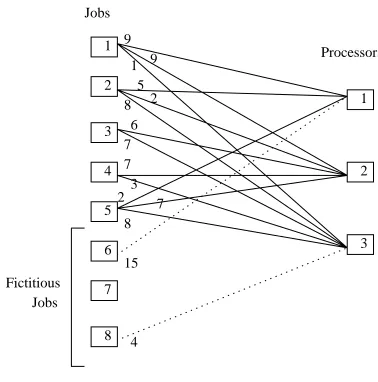
The algorithm constructs a bipartite graph, it consists of two vertex sets X =
{J1, . . . , Jn+m} and Y ={M1, . . . , Mm}. The m jobs, {Jn+1, . . . , Jm+n}, added to the job set, represent fictitious jobs and a set of edges connectJn+j toMj, 1≤j≤m to make the sum of all incoming edges into each nodeMj equal toα. The slots during which processors are assigned to these fictitious jobs represent processor idletimes.
For every job i, its slack time is defined to be the difference between the amount of time remaining in the schedule and the amount of processing left for that job. A job is said to have become critical once its slack time goes to zero, at which time the job has to be included into the schedule for it to complete by the finish time.
in the matching finishes its processing, all non-critical jobs are removed from the matching, and augmenting paths [22] from all critical jobs are computed. The symmetric difference between the current matching and the augmenting paths forms the next matching. In case the matching computed is not complete, the jobs that were removed from the previous matching are reconsidered and augmenting paths from jobs not in the current and previous matching are computed to get a complete match. The process above is repeated until the processor requirements of all the jobs is met.
[24] shows that the algorithm always has a finish time ofαand prove the correctness of the algorithm that a complete matching can be obtained during every iteration of the algorithm. The asymptotic time complexity of the algorithm isO(r(min{r, m2}+mlogn)), where n is the number of jobs, m the number of processors, and r the number of nonzero tasks.
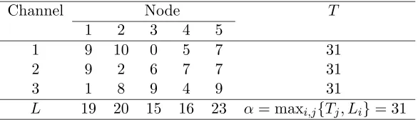
The example in Table 4.1 considers a three-processor open shop problem with five jobs and the following task times:
Processor Job T
1 2 3 4 5
1 9 5 0 0 2 16
2 9 2 6 7 7 31
3 1 8 7 3 8 27
L 19 15 13 10 17 α= maxi,j{Tj, Li}= 31
Table 4.1: Collapsed demand matrix for three processors and five jobs
Additions of the fictitious jobsJ6, J7 andJ8, introduces three more columns into Table 4.1:
15 0 0 0 0 0 0 0 4
As mentioned above, the weights assigned to the edges between the fictitious jobs and the processors represent idle slots. The entries in the additional columns suggest that processor 1 will have 15 idle slots and processor 3 will have 4 idle slots.
1 1 2 2 3 3 4 5 6 7 8 4 15 9 9 1 5 2 8 6 7 7 3 8 7 2 Jobs Processors Fictitious Jobs
Figure 4.1: Bipartite graph as constructed by the preemptive open-shop algorithm
being assigned to each of the three processors. The Figure 4.2 shows the resulting open-shop schedule. The initial matching assigns jobs, J6, J5 and J8 to processors M1, M2 and M3
respectively. At time 4, job J8 finishes its execution on processor M3, hence it is deleted from the matching and an augmenting path starting from a job (J4) not in the matching is computed. At time 7, job J4 finishes its execution on processor M3, and so does job
J5 on processor M2, augmenting paths starting from jobs not in the matching assign jobs
J4, J5 to processors M2, M3 respectively. After time 12, job J1 becomes critical and hence replaces jobJ5 on processorM3. Later at time 14, jobJ1 finishes its processing onM3, but remains critical hence is assignedM2 and jobJ5 regains processorM3. The next interesting instance is at time 21, at which jobJ2 becomes critical and is assigned processorM3. Next at time 23, job J3 becomes critical and is assigned processor M2. It should be noted that once a job becomes critical it is assigned a processor till the end of schedule.
Time slots 1 2 3 4 5 6 7 8 9 20
idle 2 5 1
5 4 1 4 3 2
idle 4 5 3
λ
λ
λ3
1
2
10 1 2 3 4 5 6 7 8 9 1 2 3 4 5 6 7 8 9 30 1
2 3
5 1
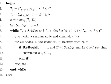
Best effort allocation for the preemptive open-shop algorithm (BE-OS)
Input: N, C, Collapsed traffic matrixA[N×C], BE requirement matrix BEReq[N×C], additional slots F
Output: Best effort allocation matrix B[N ×C] 1. begin
2. Tj = P
1≤i≤Nai,j, 1≤j≤C 3. Li=
P
1≤j≤Cai,j, 1≤i≤N 4. α= maxi,j{Tj, Li}.
5. SetSchLgt=α+F
6. whileTj < SchLgtand Li < SchLgt ∀i, j1≤i≤N, 1≤j ≤C 7. Start with a random node and channel, ri, rj
8. for all nodes,i, and channels,j, starting fromri, rj
9. if BEReq[i][j] == 1 andTj < SchLgt andLi< SchLgt then 10. increment bij, Tj, Li
11. end if
12. end for
13. end while 14. end
Figure 4.3: Algorithm: Best-effort allocation for preemptive open-shop algorithm (BE-OS)